Krylov quantum diagonalisasyon

Sa araling ito tungkol sa Krylov quantum diagonalization (KQD), sasagutin natin ang mga sumusunod:

• Ano ang paraan ng Krylov, sa pangkalahatan?
• Bakit gumagana ang paraan ng Krylov at sa anong mga kondisyon?
• Paano nakapasok ang quantum computing dito?

Ang quantum na bahagi ng mga kalkulasyon ay halaw pangunahin sa gawa sa Ref [1].

Ang video sa ibaba ay nagbibigay ng pangkalahatang-ideya ng mga paraan ng Krylov sa klasikal na computing, nagpapaliwanag ng dahilan ng paggamit nito, at nagpapaliwanag kung paano makakatulong ang quantum computing doon. Ang sumusunod na teksto ay nagbibigay ng mas detalyadong paliwanag at nagpapatupad ng isang paraan ng Krylov nang klasikal at gamit ang quantum computer.

1. Panimula sa mga paraan ng Krylov

Ang isang Krylov subspace method ay maaaring tumukoy sa alinman sa ilang mga pamamaraan na itinayo sa paligid ng tinatawag na Krylov subspace. Ang isang kumpletong pagsusuri nito ay lampas sa saklaw ng araling ito, ngunit ang Ref [2-4] ay makakapagbigay ng higit pang background. Dito, tututukan natin kung ano ang isang Krylov subspace, kung paano at bakit ito kapaki-pakinabang sa paglutas ng mga eigenvalue problem, at sa wakas kung paano ito maipapatupad sa isang quantum computer.

Kahulugan: Ibinigay ang isang simetriko, positibong semi-definite na $N\times N$ na matrix $A$, ang Krylov space $\mathcal{K}^r$ ng order na $r$ ay ang espasyong spanned ng mga vector na nakuha sa pamamagitan ng pagpaparami ng mas mataas na kapangyarihan ng matrix $A$, hanggang $r-1\leq N$, kasama ang isang reference vector na $\vert v \rangle$.

$$\mathcal{K}^r = \text{span}\left\{ \vert v \rangle, A \vert v \rangle, A^2 \vert v \rangle, ..., A^{r-1} \vert v \rangle \right\}$$

Kahit na ang mga vector sa itaas ay nag-span ng tinatawag nating Krylov subspace, walang dahilan para isipin na magiging orthogonal ang mga ito. Kadalasan ay gumagamit ng isang iterative na proseso ng orthonormalizing na katulad ng Gram-Schmidt orthogonalization. Dito ang proseso ay bahagyang naiiba dahil ang bawat bagong vector ay ginagawang orthogonal sa mga nauna habang ito ay nalilikha. Sa kontekstong ito tinatawag itong Arnoldi iteration. Simula sa paunang vector na $|v\rangle$, nililikha ang susunod na vector na $A|v\rangle$, at pagkatapos ay tinitiyak na ang pangalawang vector na ito ay orthogonal sa una sa pamamagitan ng pagbabawas ng proyeksyon nito sa $|v\rangle$. Iyon ay

$$\begin{aligned} |v_0\rangle &=\frac{|v\rangle}{\left|\left| |v\rangle \right|\right|}\\ |v_1\rangle &=\frac{A|v\rangle-\langle v_0|A|v\rangle |v_0\rangle}{\left|\left|A|v\rangle-\langle v_0|A|v\rangle |v_0\rangle \right|\right|} \end{aligned}$$

Madali na ngayong makita na $|v_0\rangle \perp |v_1\rangle,$ dahil

$$\langle v_0 | v_1\rangle=\frac{\langle v_0 | A|v\rangle-\langle v_0 |A|v\rangle\langle v_0|v_0\rangle}{\left|\left| A|v\rangle-\langle A|v\rangle|v_0\rangle |v_0\rangle \right|\right|}=0$$

Ginagawa natin ang parehong bagay para sa susunod na vector, tinitiyak na ito ay orthogonal sa parehong mga nakaraang dalawa:

$$|v_2\rangle=\frac{A |v_1\rangle-\langle v_0|A |v_1\rangle |v_0\rangle-\langle v_1|A |v_1\rangle |v_1\rangle}{\left|\left| A |v_1\rangle-\langle v_0|A |v_1\rangle |v_0\rangle-\langle v_1|A |v_1\rangle |v_1\rangle\right|\right|}$$

Kung uulitin natin ang prosesong ito para sa lahat ng $r$ na vector, magkakaroon tayo ng kumpletong orthonormal na basis para sa isang Krylov space. Pansinin na ang proseso ng orthogonalization dito ay magreresulta sa zero kapag ang $r>m$, dahil ang $m$ na orthogonal na vector ay kailangang mag-span ng buong espasyo. Ang proseso ay magreresulta din sa zero kung ang anumang vector ay isang eigenvector ng $A$ dahil ang lahat ng kasunod na vector ay magiging mga multiple ng vector na iyon.

1.1 Isang simpleng halimbawa: Krylov gamit ang kamay

Halina't magsagawa ng isang Krylov subspace generation sa isang napakaliit na matrix, para makita natin ang proseso. Magsisimula tayo sa isang paunang matrix $A$ na interesante sa atin:

$$A=\begin{pmatrix}4&-1&0\\-1&4&-1\\0&-1&4\end{pmatrix}$$

Para sa maliit na halimbawang ito, madali nating matutukoy ang mga eigenvector at eigenvalue kahit gamit ang kamay. Ipinapakita namin dito ang numerical na solusyon.

# Added by doQumentation — required packages for this notebook
!pip install -q matplotlib numpy qiskit qiskit-ibm-runtime scipy sympy

# One might use linalg.eigh here, but later matrices may not be Hermitian. So we use linalg.eig in this lesson.

import numpy as np

A = np.array([[4, -1, 0], [-1, 4, -1], [0, -1, 4]])
eigenvalues, eigenvectors = np.linalg.eig(A)
print("The eigenvalues are ", eigenvalues)
print("The eigenvectors are ", eigenvectors)

The eigenvalues are  [2.58578644 4.         5.41421356]
The eigenvectors are  [[ 5.00000000e-01 -7.07106781e-01  5.00000000e-01]
 [ 7.07106781e-01  1.37464400e-16 -7.07106781e-01]
 [ 5.00000000e-01  7.07106781e-01  5.00000000e-01]]

Itinatala natin ang mga ito dito para sa paghahambing sa bandang huli:

$$\begin{aligned} a_0&=2.59,&|0\rangle&=&\begin{pmatrix}1/2\\-\sqrt{2}/2\\1/2\end{pmatrix}\\ \\ a_1&=4,&|1\rangle&=&\begin{pmatrix}\sqrt{2}/2\\0\\-\sqrt{2}/2\end{pmatrix}\\ \\ a_2&=5.41,&|2\rangle&=&\begin{pmatrix}1/2\\\sqrt{2}/2\\1/2\end{pmatrix} \end{aligned}$$

Nais nating pag-aralan kung paano gumagana (o nabibigo) ang prosesong ito habang pinapataas natin ang dimensyon ng ating Krylov subspace, $r$. Para dito, ilalapat natin ang prosesong ito:

• Lumikha ng isang subspace ng buong vector space simula sa isang random na piniling vector na $|v\rangle$ (tawagan itong $|v_0\rangle$ kung ito ay normalized na, tulad ng nasa itaas).
• I-project ang buong matrix $A$ sa subspace na iyon, at hanapin ang mga eigenvalue ng projected na matrix na $\tilde{A}$.
• Palakihin ang laki ng subspace sa pamamagitan ng paglikha ng higit pang mga vector, tinitiyak na ang mga ito ay orthonormal, gamit ang isang proseso na katulad ng Gram-Schmidt orthogonalization.
• I-project ang $A$ sa mas malaking subspace at hanapin ang mga eigenvalue ng resultang matrix na $\tilde{A}$.
• Ulitin ito hanggang sa mag-converge ang mga eigenvalue (o sa toy case na ito, hanggang sa makabuo ka ng mga vector na nag-span ng buong vector space ng orihinal na matrix $A$).

Ang isang normal na implementasyon ng paraan ng Krylov ay hindi kailangang lutasin ang eigenvalue problem para sa matrix na naka-project sa bawat Krylov subspace habang ito ay nilillikha. Maaari mong itayo ang subspace ng ninanais na dimensyon, i-project ang matrix sa subspace na iyon, at i-diagonalize ang projected na matrix. Ang pag-project at pag-diagonalize sa bawat dimensyon ng subspace ay ginagawa lamang para sa pag-check ng convergence.

Dimensyon $r=1$:

Pumili tayo ng isang random na vector, halimbawa

$$|v_0\rangle=\begin{pmatrix}1\\0\\0\end{pmatrix}$$

Kung hindi pa ito normalized, i-normalize ito.

I-project na natin ang ating matrix $A$ sa subspace ng isang vector na ito:

$$\tilde{A}_0=\langle v_0| A|v_0\rangle=\begin{pmatrix}1&0&0\end{pmatrix}\begin{pmatrix}4&-1&0\\-1&4&-1\\0&-1&4\end{pmatrix}\begin{pmatrix}1\\0\\0\end{pmatrix}=(4)$$

Ito ang ating projection ng matrix sa ating Krylov subspace kapag naglalaman ito ng isang vector lamang, ang $|v_0\rangle$. Ang eigenvalue ng matrix na ito ay 4 nang walang karagdagang hakbang. Maaari nating isipin ito bilang ating zeroth-order na pagtatantya ng mga eigenvalue (sa kasong ito isa lamang) ng $A$. Kahit na ito ay isang mahinang pagtatantya, ito ay nasa tamang order of magnitude.

Dimensyon $r=2$:

Lilikha tayo ngayon ng susunod na vector sa ating subspace sa pamamagitan ng operasyon gamit ang $A$ sa nakaraang vector:

$$A|v_0\rangle=\begin{pmatrix}4&-1&0\\-1&4&-1\\0&-1&4\end{pmatrix}\begin{pmatrix}1\\0\\0\end{pmatrix}=\begin{pmatrix}4\\-1\\0\end{pmatrix}$$

Ibabawas na natin ang proyeksyon ng vector na ito sa ating nakaraang vector para matiyak ang orthogonality.

$$|v_1\rangle=A|v_0\rangle-\langle v_0 |A|v_0\rangle|v_0\rangle$$ $$|v_1\rangle=\begin{pmatrix}4\\-1\\0\end{pmatrix}-\begin{pmatrix}1& 0& 0\end{pmatrix}\begin{pmatrix}4\\-1\\0\end{pmatrix}\begin{pmatrix}1\\0\\0\end{pmatrix}=\begin{pmatrix}0\\-1\\0\end{pmatrix}$$

Kung hindi pa ito normalized, i-normalize ito. Sa kasong ito, ang vector ay normalized na, kaya

$$|v_1\rangle=\begin{pmatrix}0\\-1\\0\end{pmatrix}$$

I-project na natin ang ating matrix A sa subspace ng dalawang vector na ito:

$$\tilde{A}_1= \begin{pmatrix} 1&0&0\\0&-1&0 \end{pmatrix} \begin{pmatrix}4&-1&0\\-1&4&-1\\0&-1&4\end{pmatrix}\begin{pmatrix}1&0\\0&-1\\0&0\end{pmatrix}=\begin{pmatrix}1&0&0\\0&-1&0\end{pmatrix}\begin{pmatrix}4&1\\-1&-4\\0&1\end{pmatrix}=\begin{pmatrix}4&1\\1&4\end{pmatrix}$$

Nananatili pa rin tayong may problema sa pagtukoy ng mga eigenvalue ng matrix na ito. Ngunit ang matrix na ito ay bahagyang mas maliit kaysa sa buong matrix. Sa mga problemang may napakalalim na mga matrix, ang pagtatrabaho sa mas maliit na subspace na ito ay maaaring maging lubhang kapaki-pakinabang.

$$\det(\tilde{A_1}-\lambda I)=0$$ $$\begin{vmatrix} 4-\lambda&1\\1&4-\lambda\end{vmatrix} =(4-\lambda)^2-1=0$$ $$4-\lambda=±1→\lambda=3,5$$

Kahit na hindi pa rin ito isang magandang pagtatantya, mas mabuti ito kaysa sa zeroth order na pagtatantya. Isasagawa natin ito para sa isa pang iterasyon, para matiyak na malinaw ang proseso. Gayunpaman, nasisira nito ang punto ng pamamaraan, dahil magdi-diagonalize tayo ng isang 3x3 na matrix sa susunod na iterasyon, ibig sabihin ay hindi tayo nakatipid ng oras o computational power.

Dimensyon $r=3$:

Lilikha tayo ngayon ng susunod na vector sa ating subspace sa pamamagitan ng operasyon gamit ang A sa nakaraang vector:

$$A|v_1\rangle=\begin{pmatrix}4&-1&0\\-1&4&-1\\0&-1&4\end{pmatrix}\begin{pmatrix}0\\-1\\0\end{pmatrix}=\begin{pmatrix}1\\-4\\1\end{pmatrix}$$

Ibabawas na natin ang proyeksyon ng vector na ito sa parehong ating mga nakaraang vector para matiyak ang orthogonality.

$$\begin{aligned} |v_2\rangle&=A|v_1\rangle-\langle v_0 |A|v_1\rangle|v_0\rangle-\langle v_1 |A|v_1\rangle|v_1\rangle\\ |v_2\rangle&=\begin{pmatrix}1\\-4\\1\end{pmatrix}-\begin{pmatrix}1& 0& 0 \end{pmatrix}\begin{pmatrix}1\\-4\\1\end{pmatrix}\begin{pmatrix}1\\0\\0\end{pmatrix}-\begin{pmatrix}0&-1& 0\end{pmatrix}\begin{pmatrix}1\\-4\\1\end{pmatrix}\begin{pmatrix}0\\-1\\0\end{pmatrix}=\begin{pmatrix}0\\0\\1\end{pmatrix} \end{aligned}$$

Kung hindi pa ito normalized, i-normalize ito. Sa kasong ito, ang vector ay normalized na, kaya

$$|v_2 \rangle=\begin{pmatrix}0\\0\\1\end{pmatrix}$$

I-project na natin ang ating matrix $A$ sa subspace ng mga vector na ito:

$$\tilde{A}_2=\begin{pmatrix}1&0&0\\0&-1&0\\0&0&1\end{pmatrix}\begin{pmatrix}4&-1&0\\-1&4&-1\\0&-1&4\end{pmatrix}\begin{pmatrix}1&0&0\\0&-1&0\\0&0&1\end{pmatrix}=\begin{pmatrix}4&-1&0\\1&-4&1\\0&-1&4\end{pmatrix}\begin{pmatrix}1&0&0\\0&-1&0\\0&0&1\end{pmatrix}=\begin{pmatrix}4&1&0\\1&4&1\\0&1&4\end{pmatrix}$$

Tutukuyin na natin ngayon ang mga eigenvalue:

$$\det(\tilde{A}_2-\lambda I)=0$$ $$\begin{vmatrix}4-\lambda&1&0\\1&4-\lambda&1\\0&1&4-\lambda\end{vmatrix} = (4-\lambda)((4-\lambda)^2-1)-(4-\lambda)=0\\$$ $$4-\lambda=0,4-\lambda=±2^{1/2}→\lambda=4-2^{1/2},4,4+2^{1/2}≈2.59,4,5.41$$

Ang mga eigenvalue na ito ay eksaktong mga eigenvalue ng orihinal na matrix $A$. Ito ay dapat na ganito, dahil pinalawak na natin ang ating Krylov subspace para mag-span ng buong vector space ng orihinal na matrix $A$.

Sa halimbawang ito, ang paraan ng Krylov ay maaaring hindi lilitaw na mas madali kaysa sa direktang diagonalization. Sa katunayan, tulad ng makikita natin sa mga susunod na seksyon, ang paraan ng Krylov ay magiging kapaki-pakinabang lamang sa itaas ng isang tiyak na dimensyon ng matrix; ito ay nilalayong tulungan tayong lutasin ang mga eigenvalue/eigenvector problem ng napakalalim na mga matrix.

Ito lamang ang halimbawa na aming ipapakita na ginawa "gamit ang kamay", ngunit ang seksyon 2 sa ibaba ay nagpapakita ng mga computational na halimbawa.

Paglilinaw ng mga termino

Isang karaniwang maling paniniwala ay mayroon lamang isang Krylov subspace para sa isang ibinigay na problema. Ngunit siyempre, dahil maraming paunang vector kung saan maaaring ilapat ang ating matrix, maraming posibleng Krylov subspace. Gagamitin lamang natin ang pariralang "ang Krylov subspace" para tumukoy sa isang tiyak na Krylov subspace na tinukoy na para sa isang tiyak na halimbawa. Para sa mga pangkalahatang diskarte sa paglutas ng problema, titukuyin natin ito bilang "isang Krylov subspace". Isang panghuling paglilinaw ay valid na tumukoy sa isang "Krylov space". Madalas itong tinatawag na "Krylov subspace" dahil sa paggamit nito sa konteksto ng pag-project ng mga matrix mula sa isang paunang espasyo papunta sa isang subspace. Ayon sa kontekstong iyon, pangunahin nating tatawagin ito bilang isang subspace dito.

Suriin ang iyong pag-unawa

Ipaliwanag kung bakit hindi (a) kapaki-pakinabang, at (b) posible na palawakin ang dimensyon ng Krylov subspace $r$ nang higit pa sa dimensyon $N$ ng matrix na pinag-aaralan.

Answer

(a) Dahil ino-orthonormalize natin ang mga vector habang nililikha ang mga ito, ang isang hanay ng $N$ na ganoong mga vector ay bumubuo ng kumpletong basis, ibig sabihin ay maaaring gumamit ng linear na kumbinasyon ng mga ito para lumikha ng anumang vector sa espasyo.

(b) Ang proseso ng orthogonalization ay binubuo ng pagbabawas ng proyeksyon ng isang bagong vector sa lahat ng nakaraang mga vector. Kung ang lahat ng nakaraang mga vector ay nag-span ng buong vector space, ang pagbabawas ng mga proyeksyon sa buong subspace ay palaging mag-iiwan sa atin ng isang zero vector.

Ipagpalagay na ang isang kapwa mananaliksik ay nagpapapakita ng paraan ng Krylov na inilapat sa isang maliit na toy matrix. May mali ba sa kanyang pagpili ng matrix $A$ at paunang vector $|\psi\rangle$?

$$A=\begin{pmatrix}2&1&3\\1&2&3\\3&3&5\end{pmatrix}$$

at

$$|\psi\rangle=\frac{1}{\sqrt{2}}\begin{pmatrix}1\\-1\\0\end{pmatrix}.$$

Answer

Aksidente na pinili ng iyong kasamahan ang isang eigenvector bilang kanyang/niya paunang vector. Ang pagkilos gamit ang matrix sa paunang vector ay magbabalik lamang ng parehong vector, na na-scale ng eigenvalue. Hindi ito makakabuo ng subspace ng dumaraming dimensyon. Payuhan ang iyong kasamahan na pumili ng ibang paunang vector, tinitiyak na hindi ito isang eigenvector.

Ilapat ang paraan ng Krylov sa ibinigay na matrix, pumili ng angkop na bagong paunang vector. Isulat ang mga pagtatantya ng pinakamaliit na eigenvalue sa ika-0 at ika-1 na order ng iyong Krylov subspace.

$$A=\begin{pmatrix}1&1&0\\1&1&1\\0&1&1\end{pmatrix}$$

Answer

Maraming posibleng sagot depende sa pagpili ng paunang vector. Pipiliin natin ang:

$$|v_0\rangle=\frac{1}{\sqrt{3}}\begin{pmatrix}1\\1\\1\end{pmatrix}.$$

Para makuha ang $|v_1\rangle$ inilalapat natin ang $A$ nang isang beses sa $|v_0\rangle$, at pagkatapos ay ginagawang orthogonal ang $|v_1\rangle$ sa $|v_0\rangle.$

$$A|v_0\rangle=\begin{pmatrix}1&1&0\\1&1&1\\0&1&1\end{pmatrix}\frac{1}{\sqrt{3}}\begin{pmatrix}1\\1\\1\end{pmatrix} = \frac{1}{\sqrt{3}}\begin{pmatrix}2\\3\\2\end{pmatrix}$$$$A|v_0\rangle - \langle v_0|A|v_0\rangle |v_0\rangle=\frac{1}{\sqrt{3}}\begin{pmatrix}2\\3\\2\end{pmatrix} - \frac{1}{\sqrt{3}}\begin{pmatrix}1&1&1\end{pmatrix}\frac{1}{\sqrt{3}}\begin{pmatrix}2\\3\\2\end{pmatrix}\frac{1}{\sqrt{3}}\begin{pmatrix}1\\1\\1\end{pmatrix} = \frac{1}{\sqrt{3}}\begin{pmatrix}2\\3\\2\end{pmatrix}-\frac{7}{3}\frac{1}{\sqrt{3}}\begin{pmatrix}1\\1\\1\end{pmatrix}=\sqrt{\frac{3}{2}}\begin{pmatrix}-1/3\\2/3\\-1/3\end{pmatrix}$$

Sa ika-0 na order, ang projection sa ating Krylov subspace ay

$$\langle v_0|A|v_0\rangle=\frac{1}{\sqrt{3}}\begin{pmatrix}1&1&1\end{pmatrix} \begin{pmatrix}1&1&0\\1&1&1\\0&1&1\end{pmatrix} \frac{1}{\sqrt{3}}\begin{pmatrix}1\\1\\1\end{pmatrix} = \frac{7}{3}$$

Sa ika-1 na order, ang projection sa Krylov subspace na ito ay

$$\langle V^1|A|V^1\rangle=\begin{pmatrix}\frac{1}{\sqrt{3}}&\frac{1}{\sqrt{3}}&\frac{1}{\sqrt{3}}\\-\sqrt{\frac{1}{6}}&\sqrt{\frac{2}{3}}&-\sqrt{\frac{1}{6}}\end{pmatrix} \begin{pmatrix}1&1&0\\1&1&1\\0&1&1\end{pmatrix} \begin{pmatrix}\frac{1}{\sqrt{3}}&-\sqrt{\frac{1}{6}}\\\frac{1}{\sqrt{3}}& \sqrt{\frac{2}{3}} \\ \frac{1}{\sqrt{3}}&-\sqrt{\frac{1}{6}}\end{pmatrix}$$

Maaari itong gawin gamit ang kamay, ngunit pinakamadaling gawin gamit ang numpy:

import numpy as np
vstar = np.array([[1/np.sqrt(3),1/np.sqrt(3),1/np.sqrt(3)],[-1/np.sqrt(6),np.sqrt(2/3),-1/np.sqrt(6)]]
)
A = np.array([[1, 1, 0],
              [1, 1, 1],
              [0, 1, 1]])
v = np.array([[1/np.sqrt(3),-1/np.sqrt(6)],[1/np.sqrt(3),np.sqrt(2/3)],[1/np.sqrt(3),-1/np.sqrt(6)]])
proj = vstar@A@v
print(proj)
eigenvalues, eigenvectors = np.linalg.eig(proj)
print("The eigenvalues are ", eigenvalues)
print("The eigenvectors are ", eigenvectors)

output:

[[ 2.33333333  0.47140452]
 [ 0.47140452 -0.33333333]]
The eigenvalues are  [ 2.41421356 -0.41421356]
The eigenvectors are  [[ 0.98559856 -0.16910198]
 [ 0.16910198  0.98559856]]

Ang pinakamaliit na pagtatantya ng eigenvalue ay -0.414.

1.2 Mga uri ng paraan ng Krylov

Ang "Krylov subspace methods" ay maaaring tumukoy sa alinman sa ilang iterative na pamamaraan na ginagamit upang malutas ang malalaking linear system at eigenvalue problem. Ang mayroon silang lahat ay gumagawa sila ng approximate na solusyon mula sa isang Krylov subspace

$\mathcal{K}^r(A,|v\rangle ) = \text{span}\{|v\rangle, A|v\rangle, A^2|v\rangle, ..., A^{r-1}|v\rangle\},$

kung saan ang $|v\rangle$ ay ang paunang hula (tingnan ang Ref [5]). Naiiba sila sa kung paano nila pinipili ang pinakamahusay na approximation mula sa subspace na ito, binabago ang mga salik tulad ng convergence rate, paggamit ng memory, at kabuuang computational cost. Ang pokus ng araling ito ay ang samantalahin ang quantum computing sa konteksto ng Krylov subspace methods; ang isang exhaustive na talakayan ng mga pamamaraang ito ay lampas sa saklaw nito. Ang mga maikling kahulugan sa ibaba ay para sa konteksto lamang at may kasamang ilang sanggunian para sa pagsisiyasat ng mga pamamaraang ito nang higit pa.

Ang conjugate gradient (CG) method: Ang pamamaraang ito ay ginagamit para sa paglutas ng mga simetriko, positibong definitong linear system[6]. Inililimitahan nito ang A-norm ng error sa bawat iterasyon, na ginagawa itong epektibo para sa mga sistema na nagmumula sa mga discretized elliptic PDE[7]. Gagamitin natin ang diskarteng ito sa susunod na seksyon para motibahin ang dahilan kung bakit ang isang Krylov subspace ay magiging isang epektibong subspace kung saan maaari tayong maghanap ng mas magandang solusyon sa mga linear system.

Ang generalized minimal residual (GMRES) method: Ito ay dinisenyo para sa paglutas ng mga pangkalahatang non-simetriko na linear system. Inililimitahan nito ang residual norm sa isang Krylov space sa bawat iterasyon, na ginagawa itong matibay ngunit potensyal na memory-intensive para sa malalaking sistema[7].

Ang minimal residual (MINRES) method: Ang pamamaraang ito ay ginagamit para sa paglutas ng mga simetriko, indefinite na linear system. Katulad ito ng GMRES ngunit sinasamantala ang simetrya ng matrix para mabawasan ang computational cost[8].

Ang iba pang mga diskarteng kapansin-pansin ay kinabibilangan ng full orthogonalization method (FOM), na malapit na kaugnay ng paraan ni Arnoldi para sa mga eigenvalue problem, ang bi-conjugate gradient (BiCG) method, at ang induced dimension reduction (IDR) method.

1.3 Bakit gumagana ang Krylov subspace method

Dito, ipamumotibahin natin na ang Krylov subspace method ay dapat na isang mahusay na paraan para ma-approximate ang mga eigenvalue ng matrix sa pamamagitan ng iterative refinement ng mga approximation ng eigenvector, sa pamamagitan ng lente ng steepest descent. Itatalo natin na, ibinigay ang isang paunang hula ng isang ground state, ang espasyo ng mga sunud-sunod na correksyon sa paunang hulang iyon na nagbubunga ng pinakamabilis na convergence ay isang Krylov subspace. Titigil tayo sa isang mahigpit na patunay ng gawi ng convergence.

Ipagpalagay na ang ating matrix na pinag-aaralan na $A$ ay simetriko at positibong definite. Ginagawa nitong pinaka-angkop ang ating argumento sa CG method sa itaas. Walang mga pagpapalagay na ginagawa tungkol sa sparsity dito; ni hindi tayo nagsasabing ang $A$ ay dapat na Hermitian (na kailangan nito kung ito ay isang Hamiltonian).

Karaniwan nating nais na malutas ang isang problemang may anyo

$$A|x\rangle=|b\rangle.$$

Maaaring isipin ng isa na ang $|b\rangle=c|x\rangle$ kung saan ang $c$ ay ilang constant, tulad ng sa isang eigenvalue problem. Ngunit ang ating pahayag ng problema ay nananatiling mas pangkalahatan sa ngayon.

Magsisimula tayo sa isang vector na $|x_0\rangle$ na isang approximate na solusyon. Kahit may mga pagkakatulad sa pagitan ng hulang $|x_0\rangle$ na ito at ng $|v_0\rangle$ sa Seksyon 1.1, hindi natin ito ginagamit dito. Ang ating hulang $|x_0\rangle$ ay may error, na tinatawag nating $|e_0\rangle:$

$$|e_0\rangle:=|x\rangle−|x_0\rangle.$$

Tinutukoy din natin ang residual na $R_0:$

$$|R_0\rangle=|b\rangle−A|x_0\rangle.$$

Dito ay gumagamit tayo ng malalaking titik na $R$ para mapaghiwalatig ang residual mula sa dimensyon ng ating Krylov subspace $r$.

Nais na nating gumawa ng isang hakbang ng correksyon na may anyo

$$|x_1\rangle=|x_0\rangle+|p_0\rangle,$$

na umaasa nating mapapabuti ang ating approximation. Dito ang $|p_0\rangle$ ay ilang vector na hindi pa natutukoy. Hayaan ang $|e_1\rangle$ na maging error pagkatapos gawin ang correksyon. Pagkatapos

$$|e_1\rangle=|x\rangle−|x_1\rangle=|x\rangle−(|x_0\rangle+|p_0\rangle)=|e_0\rangle−|p_0\rangle.$$

Interesado tayo sa kung paano kumikilos ang ating error kapag na-transform ng ating matrix. Kaya kalkulahin natin ang $A$-norm ng error. Iyon ay

$$\begin{aligned} ∥|e_0\rangle−|p_0\rangle∥_A^2&=\left(\langle e_0|A−\langle p_0|A\right)\left(|e_0\rangle−|p_0\rangle\right)\\ & = \langle e_0|A|e_0 \rangle − \langle e_0|A|p_0\rangle − \langle p_0|A|e_0\rangle+\langle p_0|A|p_0\rangle\\ & = \langle e_0|A|e_0\rangle−2\langle e_0|A|p_0\rangle+\langle p_0|A|p_0\rangle\\ & = d−2\langle R_0|p_0\rangle +\langle p_0|A|p_0\rangle, \end{aligned}$$

kung saan ginamit natin ang simetrya ng $A$ at pati na rin ang $A |e_0\rangle = |R_0\rangle.$ Dito ang $d$ ay ilang constant na independiyente sa $|p_0\rangle$. Tulad ng nabanggit sa Seksyon 1.2, ang $A$-norm ng error ay hindi lang ang tanging dami na maaari nating piliing i-minimize, ngunit isa itong magandang pagpipilian. Nais nating makita kung paano nagbabago ang daming ito sa ating pagpili ng mga correksyon na vector na $|p_0\rangle.$ Kaya tinutukoy natin ang function na $f$ sa pamamagitan ng pagtatakda

$$f(|p_0\rangle)=\langle p_0|A|p_0\rangle−2\langle R_0|p_0\rangle+d.$$

Ang $f$ ay ang error lamang na $|e_1\rangle$ bilang isang function ng correksyon na $|p_0\rangle$ na sinusukat sa $A$-norm. Kaya naman, nais nating piliin ang $|p_0\rangle$ na ang $f(|p_0\rangle)$ ay magiging kaliit-liit. Para sa layuning ito, kinukuwenta natin ang gradient ng $f$. Gamit ang simetrya ng $A$ mayroon tayong

$$\nabla f(|p_0\rangle) = 2(A|p_0\rangle−|R_0\rangle).$$

Ang gradient ay tumuturo sa direksyon ng pinakamataas na pagtaas, ibig sabihin ang kabaligtaran nito ay nagbibigay sa atin ng direksyon kung saan pinakamabilis na bumababa ang function: ang direksyon ng steepest descent. Sa ating paunang hula na $|x_0\rangle$, kung saan ang $|p_0\rangle=0$, mayroon tayong $\nabla f(0) = -2|R_0\rangle.$ Kaya ang function na $f$ ay pinakamabilis na bumababa sa direksyon ng residual na $|R_0\rangle.$ Kaya ang ating paunang pagpili ay pinaka-makikinabang sa pagdaragdag ng vector na $|p_0\rangle=\alpha_0 |R_0\rangle$ para sa ilang scalar na $\alpha_0$.

Sa susunod na hakbang, pipili tayo, muli, ng isang vector na $|p_1\rangle$ at idadagdag ang halaga nito sa kasalukuyang approximation. Gamit ang parehong argumento tulad ng dati ay pipiliin natin ang $|p_1\rangle = \alpha_1 |R_1\rangle$ para sa ilang scalar na $\alpha_1$. Magpapatuloy tayo sa ganitong paraan, upang ang $k^\text{th}$ na iterasyon ng ating vector ay

$$|x_{k+1}\rangle=|x_0\rangle+\alpha_0 |R_0\rangle+\alpha_1 |R_1\rangle+⋯+\alpha_k |R_k\rangle.$$

Katumbas nito, nais naming itayo ang espasyo kung saan pinipili natin ang ating mga pinahusay na pagtatantya sa pamamagitan ng pagdaragdag ng $|R_0\rangle$, $|R_1\rangle$, at iba pa, sa pagkakasunud-sunod. Ang $k^\text{th}$ na estimated vector ay nasa loob ng

$$|x_{k+1}\rangle\in |x_0\rangle+\text{span}\{|R_0\rangle,|R_1\rangle,…,|R_k\rangle \}.$$

Ngayon, gamit ang relasyon na

$$|R_{k+1}\rangle=|b\rangle−A |x_{k+1}\rangle=|b\rangle−A(|x_k\rangle+\alpha_k |R_k\rangle)=|R_k\rangle−\alpha_k A |R_k\rangle,$$

makikita natin na

$$\text{span} \{|R_0\rangle,|R_1\rangle,…,|R_k\rangle \}=\text{span} \{|R_0\rangle,A|R_0\rangle,…,A^{k}|R_0\rangle \}.$$

Iyon ay, ang espasyong itinatatayo natin na pinaka-mahusay na nag-a-approximate sa tamang solusyon na $|x\rangle$ ay eksaktong ang espasyong itinatatayo ng magkakasunod na operasyon ng matrix $A$ sa $|R_0\rangle.$ Ang isang Krylov subspace ay ang espasyong spanned ng mga vector ng magkakasunod na direksyon ng steepest descent.

Sa wakas ay uulitin natin na walang mga numerical na pahayag na ginawa natin tungkol sa scaling ng diskarteng ito, ni hindi natin pinag-usapan ang komparatibong benepisyo para sa mga sparse matrix. Ito ay para lamang motibahin ang paggamit ng mga Krylov subspace method, at magdagdag ng ilang intuitive na pag-unawa sa mga ito. Susuriin na natin ngayon ang gawi ng mga pamamaraang ito nang numerically.

Suriin ang iyong pag-unawa

Sa workflow sa itaas, iminungkahi nating i-minimize ang $A$-norm ng error. Anong iba pang mga dami ang maaaring isaalang-alang sa paghahanap ng ground state at ang eigenvalue nito?

Answer

Maaaring isipin ng isa ang paggamit ng residual vector sa halip ng $A$-norm ng error. Maaaring may mga kaso kung saan ang pagsasaalang-alang sa error vector mismo ay kapaki-pakinabang.

2. Mga pamamaraan ng Krylov sa klasikal na computation

Sa seksyong ito, ipapatupad natin ang mga Arnoldi iteration sa pamamagitan ng code para magamit ang isang Krylov subspace sa paglutas ng mga eigenvalue problem. Ilalapat natin ito una sa isang maliit na halimbawa, pagkatapos ay titingnan kung paano lumalaki ang oras ng computation habang lumalaki ang sukat ng matrix. Isang mahalagang ideya dito ang pagbuo ng mga vector na sumasaklaw sa Krylov space — ito ang pinakamalaking kontribyutor sa kabuuang oras ng computation. Ang kinakailangang memorya ay magbabago depende sa partikular na pamamaraan ng Krylov. Ngunit ang mga limitasyon sa memorya ay maaaring humadlang sa paggamit ng mga tradisyonal na pamamaraan ng Krylov.

2.1 Simpleng maliit na halimbawa

Sa proseso ng paglikha ng Krylov subspace, kailangan nating i-orthonormalize ang mga vector sa ating subspace. Tukuyin natin ang isang function na tumatanggap ng isang kilalang vector mula sa ating subspace na vknown (hindi inaasumeng normalized) at isang kandidatong vector na idadagdag sa ating subspace na vnext, at gagawin nitong vnext na ortogonal sa vknown at ma-normalize. Tukuyin din natin ang isang function na dumadaan sa prosesong ito para sa lahat ng naitatag na vector sa ating Krylov subspace upang matiyak ang isang ganap na orthonormal na set.

# vknown is some established vector in our subspace. vnext is one we wish to add, which must be orthogonal to vknown.

def orthog_pair(vknown, vnext):
    vknown = vknown / np.sqrt(vknown.T @ vknown)
    diffvec = vknown.T @ vnext * vknown
    vnext = vnext - diffvec
    return vnext

# v is the candidate vector to be added to our subspace. s is the existing subspace.

def orthoset(v, s):
    v = v / np.sqrt(v.T @ v)
    temp = v
    for i in range(len(s)):
        temp = orthog_pair(s[i], temp)
    v = temp / np.sqrt(temp.T @ temp)
    return v

Ngayon, tukuyin natin ang isang function na nagtatayo ng unti-unting lumalaki pang Krylov subspace, hanggang ang espasyo ng mga Krylov vector ay sumasaklaw sa buong espasyo ng orihinal na matrix. Ito ay magbibigay-daan sa atin na makita kung gaano kahusay ang mga eigenvalue na nakuha gamit ang ating Krylov subspace method kumpara sa eksaktong mga halaga, bilang isang function ng dimensyon ng Krylov subspace. Mahalaga, ibinabalik ng ating function na krylov_full_build ang mga Krylov vector, ang mga projected na Hamiltonian, ang mga eigenvalue, at ang kinakailangang oras.

# Necessary imports and definitions to track time in microseconds
import time

def time_mus():
    return int(time.time() * 1000000)

# This function constructs a Krylov subspace that spans the whole space of the original matrix.
#     Input:
#       v0          : initial vector
#       matrix      : original matrix to be diagonalized
#     Output:
#       ks          : Krylov vectors
#       Hs          : projected Hamiltonians
#       eigs        : eigenvalues
#       k_tot_times : time required for the operation

def krylov_full_build(v0, matrix):
    t0 = time_mus()
    b = v0 / np.sqrt(v0 @ v0.T)
    A = matrix
    ks = []
    ks.append(b)
    Hs = []
    eigs = []
    Hs.append(b.T @ A @ b)
    eigs.append(np.array([b.T @ A @ b]))
    k_tot_times = []

    for j in range(len(A) - 1):
        vec = A @ ks[j].T
        ortho = orthoset(vec, ks)
        ks.append(ortho)
        ksarray = np.array(ks)
        Hs.append(ksarray @ A @ ksarray.T)
        eigs.append(np.linalg.eig(Hs[j + 1]).eigenvalues)
        k_tot_times.append(time_mus() - t0)

    # Return the Krylov vectors, the projected Hamiltonians, the eigenvalues, and the total time required.
    return (ks, Hs, eigs, k_tot_times)

Susubukan natin ito sa isang matrix na maliit pa rin, ngunit mas malaki na kaysa sa gusto nating gawin nang mano-mano.

# Define our small test matrix
test_matrix = np.array(
    [
        [4, -1, 0, 1, 0],
        [-1, 4, -1, 2, 1],
        [0, -1, 4, 3, 3],
        [1, 2, 3, 4, 0],
        [0, 1, 3, 0, 4],
    ]
)

# Give the test matrix and an initial guess as arguments in the function defined above. Calculate outputs.
test_ks, test_Hs, test_eigs, text_k_tot_times = krylov_full_build(
    np.array([0.5, 0.5, 0, 0.5, 0.5]), test_matrix
)

Maaari nating suriin ang ating mga function sa pamamagitan ng pagtiyak na sa huling hakbang (kapag ang Krylov space ay ang buong vector space ng orihinal na matrix) ang mga eigenvalue mula sa pamamaraan ng Krylov ay eksaktong tumutugma sa mga mula sa eksaktong numerical na diagonalization:

print(np.linalg.eig(test_matrix).eigenvalues)
print(test_eigs[len(test_matrix) - 1])

[-1.36956923  8.43756009  2.9040308   5.34436028  4.68361806]
[-1.36956923  8.43756009  2.9040308   4.68361806  5.34436028]

Matagumpay iyon. Siyempre, ang tunay na mahalaga ay kung gaano kahusay ang ating pagtatantya bilang isang function ng dimensyon ng ating Krylov subspace. Dahil madalas tayong interesado sa paghahanap ng mga ground state at iba pang pinakamababang eigenvalue (at para sa iba pang mas algebraic na dahilan na ipinaliwanag sa ibaba), tingnan natin ang ating tantya ng pinakamababang eigenvalue bilang isang function ng dimensyon ng Krylov subspace. Iyon ay

def errors(matrix, krylov_eigs):
    targ_min = min(np.linalg.eig(matrix).eigenvalues)
    err = []
    for i in range(len(matrix)):
        err.append(min(krylov_eigs[i]) - targ_min)
    return err

import matplotlib.pyplot as plt

krylov_error = errors(test_matrix, test_eigs)

plt.plot(krylov_error)
plt.axhline(y=0, color="red", linestyle="--")  # Add dashed red line at y=0
plt.xlabel("Order of Krylov subspace")  # Add x-axis label
plt.ylabel("Error in minimum eigenvalue")  # Add y-axis label
plt.show()

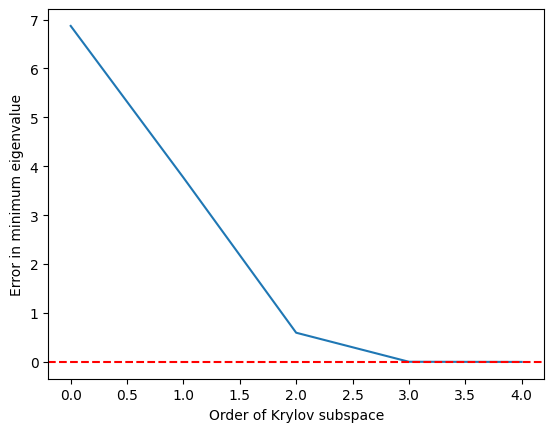
Makikita natin na ang pinakamababang eigenvalue ay naabot nang medyo tumpak kapag ang Krylov subspace ay lumaki na sa $\mathcal{K}^2,$ at perpekto na sa $\mathcal{K}^3.$

2.2 Pag-scale ng oras sa dimensyon ng matrix

Kumbinsihin natin ang ating sarili na maaaring maging kapaki-pakinabang ang pamamaraan ng Krylov kumpara sa eksaktong mga numerical eigensolver sa sumusunod na paraan:

• Bumuo ng mga random na matrix (hindi sparse, hindi ang ideal na aplikasyon para sa KQD)
• Tukuyin ang mga eigenvalue gamit ang dalawang pamamaraan: direkta gamit ang NumPy at gamit ang Krylov subspace.
• Pumili ng cutoff para sa kung gaano katumpak ang ating mga eigenvalue bago natin tanggapin ang mga Krylov na tantya.
• Ihambing ang wall time na kinakailangan para malutas sa dalawang paraan na ito.

Mga paunawa: Tulad ng tatalakayin natin nang detalyado sa ibaba, ang Krylov quantum diagonalization ay pinakamainam na inilalapat sa mga operator na ang mga matrix na representasyon ay sparse at/o maaaring isulat gamit ang maliit na bilang ng mga grupo ng commuting Pauli operator. Ang mga random na matrix na ginagamit natin dito ay hindi tumutugma sa paglalarawang iyon. Ang mga ito ay kapaki-pakinabang lamang sa pag-usisa ng sukat kung saan ang mga klasikal na pamamaraan ng Krylov ay maaaring maging kapaki-pakinabang. Pangalawa, sa paggamit ng pamamaraan ng Krylov ay magkakalkula tayo ng mga eigenvalue gamit ang maraming iba't ibang laking Krylov subspace. Iuulat natin ang oras na kinakailangan para sa pinakamaliit na dimensyong Krylov subspace na nakakamit ng ating kinakailangang katumpakan para sa ground state eigenvalue. Muli, ito ay medyo naiiba sa paglutas ng isang problema na hindi malulutas ng eksaktong mga eigensolver, dahil ginagamit natin ang eksaktong solusyon upang masuri ang kinakailangang dimensyon.

Magsisimula tayo sa pamamagitan ng pagbuo ng ating hanay ng mga random na matrix.

import numpy as np

# Set the random seed
np.random.seed(42)

# how many random matrices will we make
num_matrix = 200

matrices = []
for m in range(1, num_matrix):
    matrices.append(np.random.rand(m, m))

I-diagonalize natin ngayon ang bawat matrix nang direkta, gamit ang numpy. Kinakalkula natin ang oras na kinakailangan para sa diagonalization para sa paghahambing sa ibang pagkakataon.

matrix_numpy_times = []
matrix_numpy_eigs = []
for mm in range(num_matrix - 1):
    t0 = time_mus()
    matrix_numpy_eigs.append(min(np.linalg.eig(matrices[mm]).eigenvalues))
    matrix_numpy_times.append(time_mus() - t0)

plt.plot(matrix_numpy_times)
plt.xlabel("Dimension of matrix")  # Add x-axis label
plt.ylabel("Time to diagonalize (microsec)")  # Add y-axis label
plt.show()

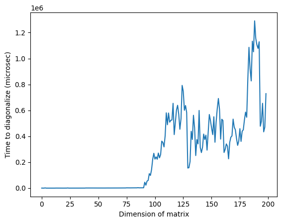
Pansinin na sa larawan sa itaas, ang hindi karaniwan na mataas na oras sa paligid ng dimensyon na 125 ay maaaring dahil sa random na katangian ng mga matrix o sa implementasyon sa klasikal na processor na ginamit, ngunit hindi ito maaaring muling gawin. Ang muling pagpapatakbo ng code ay magbibigay ng ibang profile na may iba't ibang hindi karaniwang mga taluktok.

Ngayon para sa bawat matrix, magtatayo tayo ng Krylov subspace at magkakalkula ng mga eigenvalue nang sunud-sunod. Sa bawat hakbang, susuriin natin kung ang pinakamababang eigenvalue ay nakuha na sa loob ng ating tinukoy na ganap na error. Ang subspace na unang nagbibigay sa atin ng mga eigenvalue sa loob ng ating tinukoy na error ang subspace kung saan natin itatala ang mga oras ng computation. Ang pagpapatupad ng cell na ito ay maaaring tumagal ng ilang minuto, depende sa bilis ng processor. Huwag mag-atubiling laktawan ang pagsusuri o bawasan ang maximum na dimensyon ng mga matrix na dina-diagonalize. Sapat na ang pagtingin sa mga pre-calculated na resulta.

# Choose the absolute error you can tolerate, and make a list for tracking the Krylov subspace size at which that error is achieved.
abserr = 0.05
accept_subspace_size = []

# Lists to store total time spent on the Krylov method, and the subset of that time spent on diagonalizing the projected matrix.
matrix_krylov_tot_times = []
matrix_krylov_dim = []

# Step through all our random matrices
for mm in range(0, num_matrix - 1):
    test_ks, test_Hs, test_eigs, test_k_tot_times = krylov_full_build(
        np.ones(len(matrices[mm])), matrices[mm]
    )
    # We have not yet found a Krylov subspace that produces our minimum eigenvalue to within the required error.
    found = 0
    for j in range(0, len(matrices[mm]) - 1):
        # If we still haven't found the desired subspace...
        if found == 0:
            # ...but if this one satisfies the requirement, then record everything
            if (
                abs((min(test_eigs[j]) - matrix_numpy_eigs[mm]) / matrix_numpy_eigs[mm])
                < abserr
            ):
                accept_subspace_size.append(j)
                matrix_krylov_tot_times.append(test_k_tot_times[j])
                matrix_krylov_dim.append(mm)
                found = 1

I-plot natin ang mga oras na nakuha natin para sa dalawang pamamaraang ito para sa paghahambing:

plt.plot(matrix_numpy_times, color="blue")
plt.plot(matrix_krylov_dim, matrix_krylov_tot_times, color="green")
plt.xlabel("Dimension of matrix")  # Add x-axis label
plt.ylabel("Time to diagonalize (microsec)")  # Add y-axis label
plt.show()

Ito ang aktwal na mga oras na kinakailangan, ngunit para sa layunin ng talakayan, pakinis natin ang mga curve na ito sa pamamagitan ng pag-average sa ilang mga kalapit na punto / dimensyon ng matrix. Ginagawa ito sa ibaba:

smooth_numpy_times = []
smooth_krylov_times = []

# Choose the number of adjacent points over which to average forward; the same will be used backward.
smooth_steps = 10

# We will do this smoothing for all points/matrix dimensions
for i in range(len(matrix_krylov_tot_times)):
    # Ensure we don't exceed the boundaries of our lists
    start = max(0, i - smooth_steps)
    end = min(len(matrix_krylov_tot_times) - 1, i + smooth_steps)

    # Dummy variables for accumulating an average over adjacent points. This is done for both Krylov and the NumPy calculations.
    smooth_count = 0
    smooth_numpy_sum = 0
    smooth_krylov_sum = 0

    for j in range(start, end):
        smooth_numpy_sum = smooth_numpy_sum + matrix_numpy_times[j]
        smooth_krylov_sum = smooth_krylov_sum + matrix_krylov_tot_times[j]
        smooth_count = smooth_count + 1

    # Appending the averaged adjacent values to our new smooth lists
    smooth_numpy_times.append(smooth_numpy_sum / smooth_count)
    smooth_krylov_times.append(smooth_krylov_sum / smooth_count)

plt.plot(smooth_numpy_times, color="blue")
plt.plot(smooth_krylov_times, color="green")
plt.xlabel("Dimension of matrix")  # Add x-axis label
plt.ylabel("Time to diagonalize (smoothed, microsec)")  # Add y-axis label
plt.show()

Pansinin na ang oras na kinakailangan para sa pagtatayo ng isang Krylov subspace ay unang lumalagpas sa oras na kinakailangan para sa buong diagonalization ng numpy. Ngunit habang lumalaki ang sukat ng matrix, nagiging kapaki-pakinabang ang pamamaraan ng Krylov. Totoo ito kahit na babaan pa natin ang ating katanggap-tanggap na error, ngunit ang kalamangan ay nagsisimula sa mas malaking sukat ng matrix. Ito ay sulit na pag-aralan nang mabuti.

Ang time complexity ng numerical diagonalization ay $O(n^3)$ (na may ilang pagkakaiba-iba sa pagitan ng mga algorithm). Ang time complexity ng pagbuo ng isang orthonormal na basis ng $n$ na mga vector ay $O(n^3)$ din. Kaya ang kalamangan ng pamamaraan ng Krylov ay hindi nauugnay sa paggamit ng $\it{ilang}$ orthonormal na basis, kundi sa paggamit ng isang partikular na orthonormal na basis na epektibong pinipili ang mga eigenvalue ng interes. Nakita na natin ito mula sa balangkas ng patunay sa unang seksyon ng araling ito, at ito ay kritikal para sa mga garantiya ng convergence sa mga pamamaraan ng Krylov.

Suriin natin ang ating pag-unlad hanggang ngayon:

• Para sa napakalaking mga matrix, ang pamamaraan ng Krylov subspace ay maaaring magbigay ng mga approximate na eigenvalue sa loob ng kinakailangang tolerance nang mas mabilis kaysa sa mga tradisyonal na diagonalization algorithm.
• Para sa ganitong napakalaking mga matrix, ang pagbuo ng isang Krylov subspace ang pinaka-nakakaubos ng oras na bahagi ng pamamaraan ng Krylov subspace.
• Kaya ang isang mahusay na paraan ng pagbuo ng isang Krylov subspace ay magiging lubhang mahalaga. Dito na talaga pumapasok ang quantum computer.

Suriin ang iyong pag-unawa

Tingnan ang smoothed na plot ng mga oras ng diagonalization kumpara sa dimensyon ng matrix sa itaas.

(a) Sa humigit-kumulang anong dimensyon ng matrix ang pamamaraan ng Krylov ay naging mas mabilis, ayon sa plot na ito?

(b) Anong mga aspeto ng kalkulasyon ang maaaring magbago ng dimensyong iyon kung saan ang pamamaraan ng Krylov ay nagiging mas mabilis?

Answer

(a) Maaaring mag-iba ang mga sagot kung muling patakbuhin mo ang kalkulasyon, ngunit ang pamamaraan ng Krylov ay nagiging mas mabilis sa humigit-kumulang na dimensyon na 80-85.

(b) Maraming posibleng sagot. Ang ilang mahahalagang salik ay ang katumpakan na kinakailangan natin at ang sparsity ng mga matrix na dina-diagonalize.

3. Krylov sa pamamagitan ng time evolution

Lahat ng inilarawan natin hanggang ngayon ay maaaring gawin nang klasikal. Kaya paano at kailan tayo gagamit ng quantum computer? Para sa napakalalaking mga matris, maaaring mangailangan ang Krylov method ng matagal na oras ng pagkalkula at malaking halaga ng memorya. Ang oras na kailangan para sa operasyon ng matris ng $H$ sa $|v\rangle$ ay nagse-scale nang $O(N^2)$ sa pinakamalalang kaso. Kahit ang pagpaparami ng mga sparse matris sa isang vector (ang tipikal na kaso para sa klasikal na Krylov-type na mga solver) ay may time complexity scaling na $O(N)$. Ginagawa ito para sa bawat vector na gusto natin sa ating subspace. Ang dimensyon ng subspace na $r$ ay karaniwang hindi isang malaking bahagi ng $N$, at madalas na nagse-scale nang $\log(N)$. Kaya ang pagbuo ng lahat ng mga vector ay nagse-scale nang $O(N^2 \log(N))$ sa pinakamalalang kaso. Bagama't may iba pang mga hakbang, tulad ng orthogonalization, ito ang dominanteng scaling na dapat tandaan.

Binibigyan tayo ng quantum computing ng kakayahang baguhin kung anong mga katangian ng problema ang nagtatakda ng scaling ng oras at mga resources na kailangan. Sa halip na pag-asa sa sukat ng matris na $N$ sa lahat ng dako, makikita natin ang mga bagay tulad ng bilang ng mga shots at bilang ng mga non-commuting na Pauli term na bumubuo sa Hamiltonian. Galugarin natin kung paano ito gumagana.

3.1 Time evolution

Alalahanin na ang operator na nagko-time-evolve ng isang quantum state ay $e^{-iHt/\hbar}$ (at karaniwan na, lalo na sa quantum computing, na alisin ang $\hbar$ sa notasyon). Isang paraan ng pag-unawa at maging pagsasakatuparan ng ganoong exponential function ng isang operator ay ang tingnan ang Taylor series expansion nito. Pansinin na ang operasyong ito na kumikilos sa ilang paunang vector na $|v\rangle$ ay nagbubunga ng kabuuan ng mga term na may dumaraming kapangyarihan ng $H$ na inilapat sa paunang estado. Mukhang magagawa na natin ang ating Krylov subspace sa pamamagitan ng time-evolving ng ating paunang guess state!

$$\begin{aligned} e^{-iHt/\hbar}→e^{-iHt}&≈1-iHt-\frac{(H^2 t^2)}{2}+⋯\\ e^{-iHt} |v\rangle &≈ |v\rangle-iHt|v\rangle-\frac{(H^2 t^2)}{2}|v\rangle+⋯ \end{aligned}$$

Ang caveat ay nasa pagsasakatuparan ng time evolution sa isang tunay na quantum computer. Marami sa mga term sa Hamiltonian ang hindi mag-co-commute sa isa't isa. Kaya habang ang ilang simpleng exponential operator tulad ng $e^{-iZ}$ ay tumutugma sa mga simpleng circuit, ang mga pangkalahatang Hamiltonian ay hindi. At dahil naglalaman sila ng mga non-commuting na term, hindi natin maaaring basta-basta i-decompose ang exponential sa isang product ng mga simpleng isa, tulad ng magagawa natin sa mga numero.

$$e^{-iHt}=e^{-i(H_1+H_2+⋯+H_n)t}\neq e^{-iH_1 t} e^{-iH_2 t}... e^{-iH_n t}$$

Kaya hindi ito trivial, ngunit ito ay isang well-studied na proseso sa quantum computing. Isinasagawa natin ang time-evolution sa mga quantum computer gamit ang isang prosesong tinatawag na trotterization, na sa sarili nito ay isang mayamang paksa[10]. Ngunit sa pinakamataas na antas, sa pamamagitan ng paghati ng time evolution sa napakaliit na mga hakbang, sabihin nating $m$ hakbang na may sukat na $dt$, nililimitahan natin ang mga epekto ng non-commutativity ng mga term.

$$e^{-iHt}=e^{-i(H_1+H_2+⋯+H_n )t} = (e^{-i(H_1+H_2+⋯+H_n )t/m} )^m ≈(e^{-iH_1 dt} e^{-iH_2 dt} …e^{-iH_n dt} )^m$$

kung saan ang $dt = t/m$.

Tawagin nating "power Krylov subspace" ang isang Krylov subspace ng order r na nabuo natin sa klasikal na konteksto gamit ang mga kapangyarihan ng H nang direkta.

$$\mathcal{K}_P^r (H,|v\rangle)=\text{span}\{|v\rangle,H|v\rangle,H^2 |v\rangle… H^{r-1} |v\rangle\}$$

Ngayon ay bumubuo tayo ng katulad na espasyo gamit ang unitary time-evolution operator na $U \equiv e^{-iHt}$; ito ay tatawagin nating "unitary Krylov space" na $\mathcal{K}_U^r$. Ang power Krylov subspace na $\mathcal{K}_P^r$ na ginagamit natin nang klasikal ay hindi maaaring buuin nang direkta sa isang quantum computer dahil ang $H$ ay hindi isang unitary operator. Maaaring maipakita na ang paggamit ng unitary Krylov subspace ay nagbibigay ng katulad na mga garantiya ng convergence tulad ng power Krylov subspace — specifically, ang ground state error ay nagsasara nang mahusay basta ang paunang estado na $|v\rangle$ ay may overlap sa tunay na ground state na hindi exponentially vanishing, at basta may sapat na agwat sa pagitan ng mga eigenvalue. Tingnan ang Ref [1] para sa mas tumpak na talakayan ng convergence.

Dito, ang mga kapangyarihan ng $U$ ay nagiging iba't ibang time step (ang $k^\text{th}$ kapangyarihan ng $U$ ay sumusulong ng isang oras na $k \times dt$). Maaari nating i-label ang elemento ng subspace na time-evolved para sa kabuuang oras na $k dt$ bilang $|\psi_k\rangle$.

$$\begin{aligned} U&=e^{-iHdt}\\ U^k&=e^{-iH(kdt)}\\ \mathcal{K}_U^r&=\text{span}\{|\psi\rangle,U|\psi\rangle,U^2 |\psi\rangle… U^{r-1} |\psi\rangle\} \end{aligned}$$

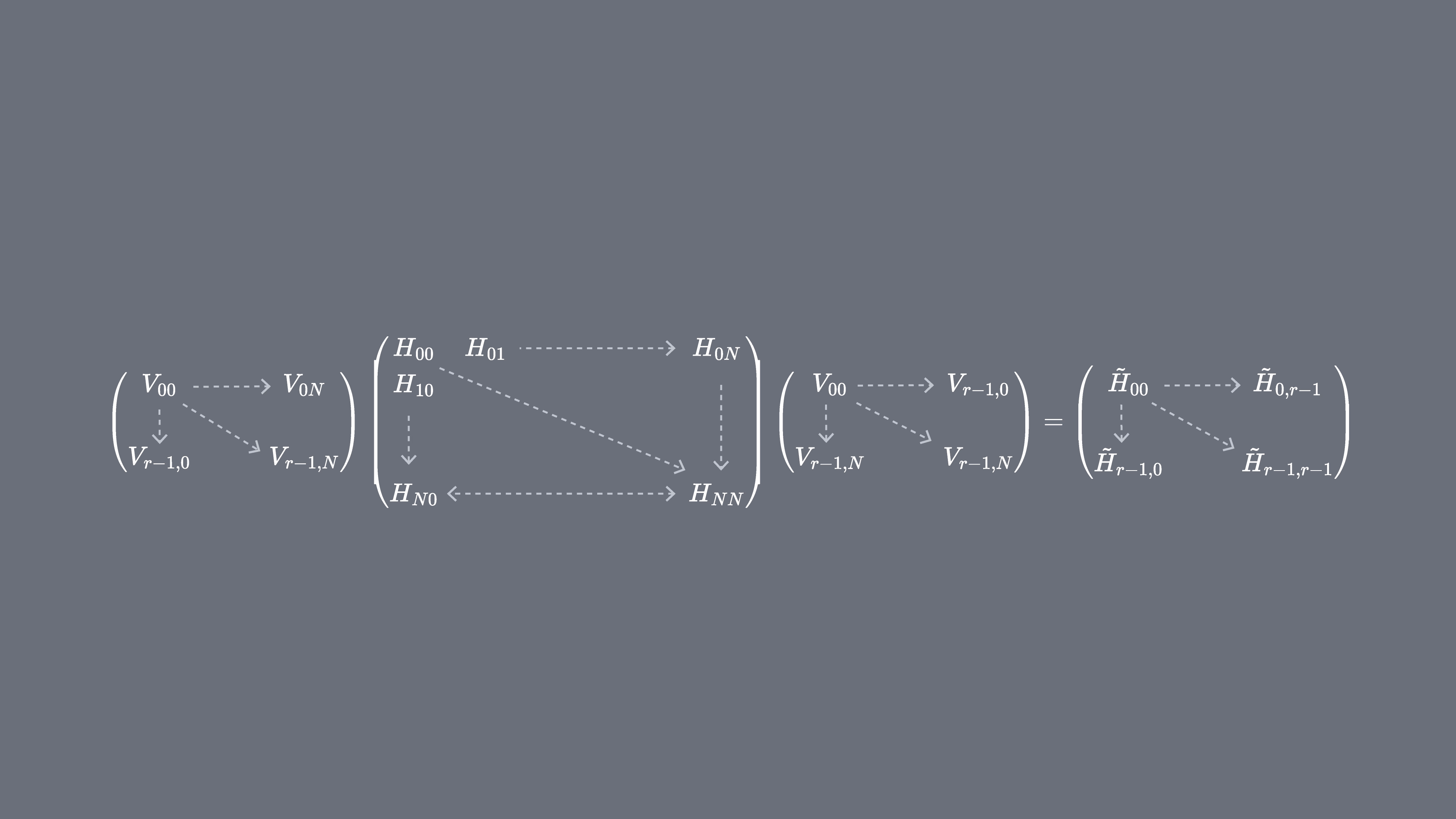
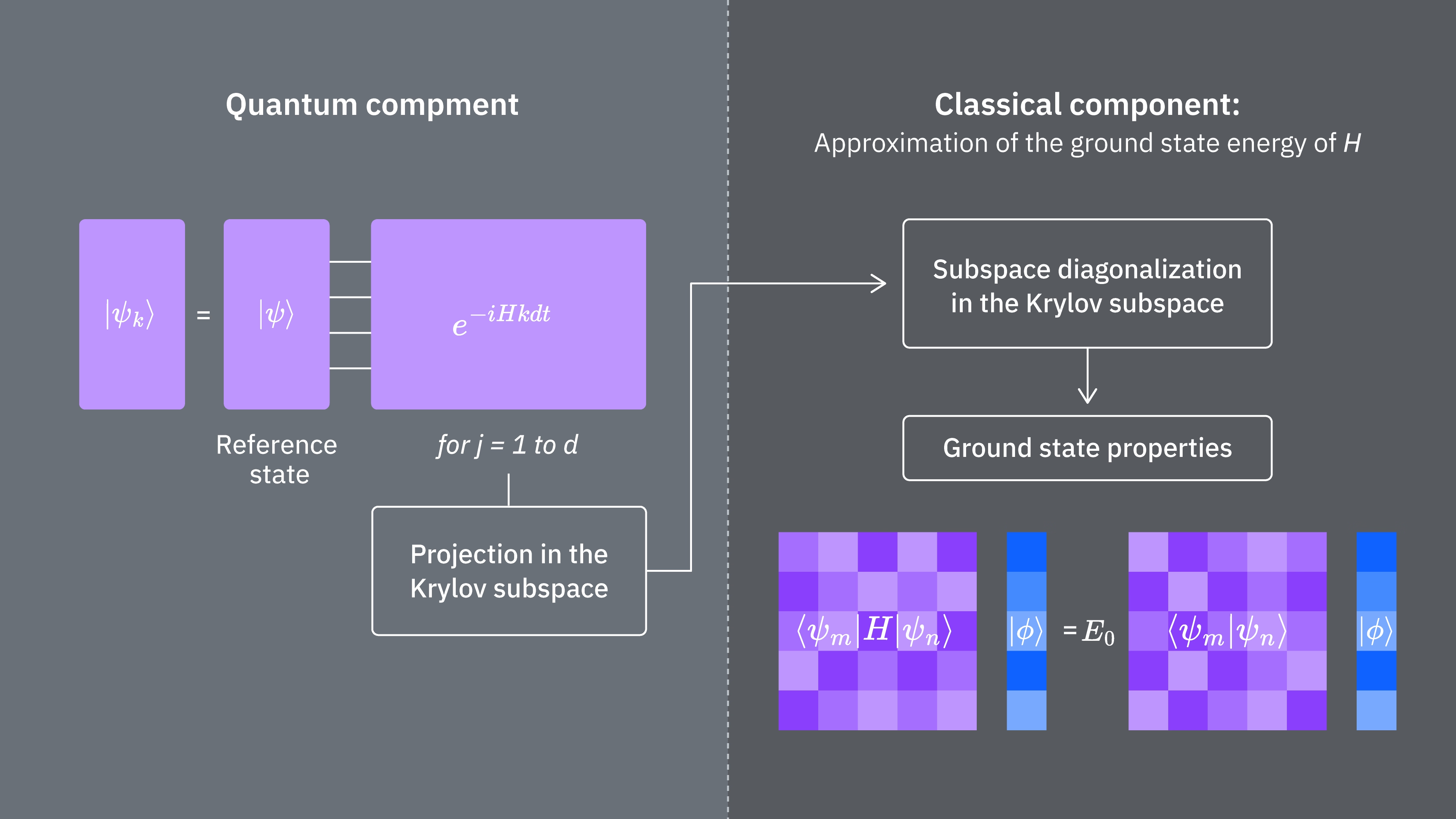
Maaari nating i-project ang ating Hamiltonian H sa unitary Krylov subspace, $\mathcal{K}_U^r$. Sa madaling salita, kinakalkula natin ang bawat matrix element ng $H$ sa basis ng $\mathcal{K}_U^r$. Tatawagin natin ang projected matrix na ito bilang $\tilde{H}$.

3.2 Paano ipapatupad sa isang quantum computer

Ang mga matrix element ng $\tilde{H}$ ay ibinibigay ng mga expectation value na $\langle \psi_m |H| \psi_n\rangle$, na maaaring matantya gamit ang quantum computer. Tandaan na ang $H$ ay maaaring isulat bilang kabuuan ng mga Pauli operator sa iba't ibang qubit, at hindi lahat ng mga Pauli operator ay maaaring sukatin nang sabay-sabay. Maaari nating ayusin ang mga Pauli term sa mga grupo ng mga commuting na term, at sukatin ang lahat ng iyon nang sabay. Ngunit maaaring kailangan ng maraming ganoong grupo upang masaklaw ang lahat ng term. Kaya ang bilang ng mga natatanging commuting na grupo kung saan maaaring mahahati ang mga term, $N_\text{GCP}$, ay nagiging mahalaga.

$$H=\sum_{\alpha=1}^{N_\text{GCP}} c_\alpha P_\alpha$$

Dito ang $P_\alpha$ ay isang Pauli string ng anyo $P_\alpha \sim IZIXII...YZXIX$ o isang set ng ganoong mga Pauli string na nag-co-commute sa isa't isa. Dahil maaari nating isulat ang $H$ bilang ganoong kabuuan ng mga measurable na operator, ang mga sumusunod na expression para sa mga matrix element ng $\tilde{H}$ ay maaaring matupad gamit ang Qiskit Runtime primitive Estimator.

$$\begin{aligned} \tilde{H}_{mn}&=\langle \psi_m |H| \psi_n\rangle\\ &=\langle \psi e^{iHt_m} |H| \psi e^{-iHt_n}\rangle\\ &=\langle \psi e^{iHmdt} |H|\psi e^{-iHndt}\rangle \end{aligned}$$

Kung saan ang $\vert \psi_n \rangle = e^{-i H t_n} \vert \psi \rangle$ ay ang mga vector ng unitary Krylov space at ang $t_n = n dt$ ay ang mga multiple ng time step na $dt$ na pinili. Sa isang quantum computer, ang pagkalkula ng bawat matrix element ay maaaring gawin gamit ang anumang algorithm na nagbibigay-daan sa atin na makuha ang overlap sa pagitan ng mga quantum state. Sa araling ito, magtutuon tayo sa Hadamard test. Dahil ang $\mathcal{K}_U$ ay may dimensyon na $r$, ang Hamiltonian na na-project sa subspace ay magkakaroon ng mga dimensyon na $r \times r$. Kung sapat na maliit ang $r$ (sa pangkalahatan ay sapat ang $r<<100$ upang makuha ang convergence ng mga tantya ng eigenvalue), maaari nating madaling i-diagonalize ang projected Hamiltonian na $\tilde{H}$ nang klasikal. Gayunpaman, hindi natin maaaring direktang i-diagonalize ang $\tilde{H}$ dahil sa non-orthogonality ng mga Krylov space vector. Kailangan nating sukatin ang kanilang mga overlap at bumuo ng matris na $\tilde{S}$

$$\tilde{S}_{mn} = \langle \psi_m \vert \psi_n \rangle$$

Nagbibigay-daan ito sa atin na malutas ang eigenvalue problem sa isang non-orthogonal na espasyo (tinatawag din na generalized eigenvalue problem)

$$\tilde{H} \ \vec{c} = E \ \tilde{S} \ \vec{c}$$

Maaari ring makuha ang mga tantya ng mga eigenvalue at eigenstate ng $H$ sa pamamagitan ng pagtingin sa mga solusyon ng generalized eigenvalue problem na ito. Halimbawa, ang tantya ng ground state energy ay nakuha sa pamamagitan ng pagkuha ng pinakamaliit na eigenvalue na $E$ at ang ground state mula sa kaukulang eigenvector na $\vec{c}$. Ang mga coefficient sa $\vec{c}$ ay nagtatakda ng kontribusyon ng iba't ibang vector na sumasaklaw sa $\mathcal{K}_U$.

Generalized eigenvalue problem

Bakit hindi natin basta-basta i-diagonalize ang $\tilde{H}$? Dahil naglalaman ang $\tilde{S}$ ng impormasyon tungkol sa geometry ng Krylov basis (na non-orthogonal sa lahat maliban sa napaka-espesyal na mga kaso), ang $\tilde{H}$ nang mag-isa ay hindi naglalarawan ng projection ng buong Hamiltonian, kaya ang mga eigenvalue nito ay walang partikular na kaugnayan sa mga eigenvalue ng buong Hamiltonian — maaari silang maging anumang random na halaga. Kailangan ang paglutas ng generalized eigenvalue problem upang makuha ang mga tinatayang eigenvalue at eigenvector na tumutugma sa projection ng buong Hamiltonian sa Krylov space.

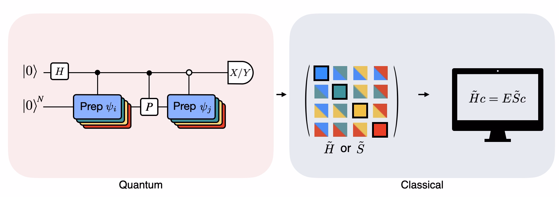
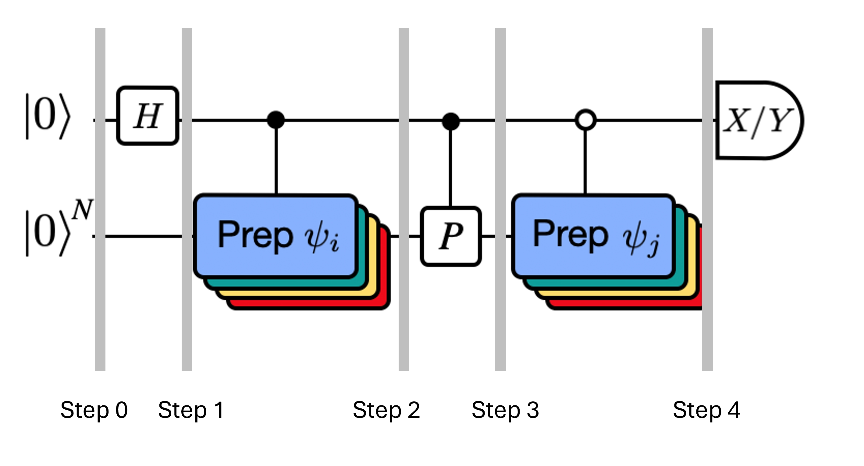
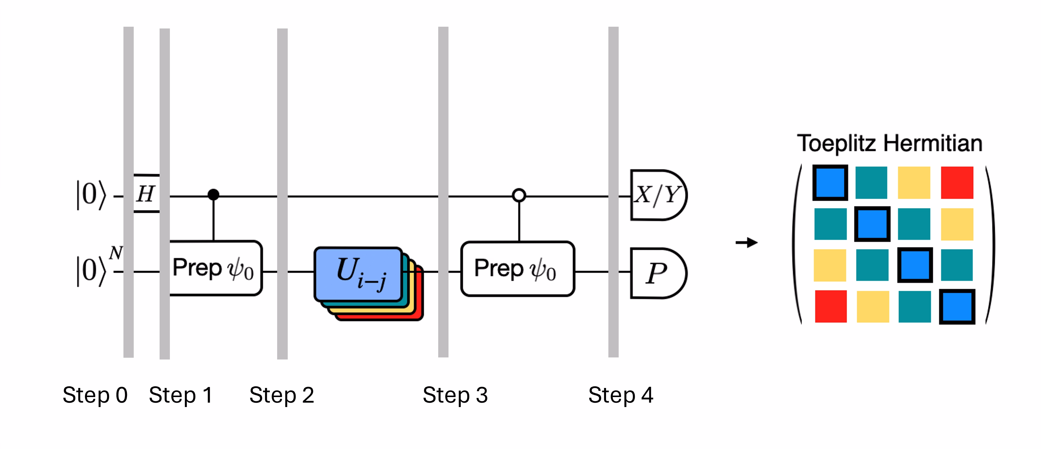
Ipinapakita ng Figure ang isang circuit representation ng modified Hadamard test, isang pamamaraan na ginagamit upang makalkula ang overlap sa pagitan ng iba't ibang quantum state. Para sa bawat matrix element na $\tilde{H}_{i,j}$, isang Hadamard test sa pagitan ng estado na $\vert \psi_i \rangle$, $\vert \psi_j \rangle$ ay isinasagawa. Naka-highlight ito sa figure sa pamamagitan ng color scheme para sa mga matrix element at ang kaukulang $\text{Prep} \; \psi_i$, $\text{Prep} \; \psi_j$ na mga operasyon. Kaya, isang set ng mga Hadamard test para sa lahat ng posibleng kombinasyon ng mga Krylov space vector ang kailangan upang makalkula ang lahat ng matrix element ng projected Hamiltonian na $\tilde{H}$. Ang tuktok na wire sa Hadamard test circuit ay isang ancilla qubit na sinusukat alinman sa X o Y basis; ang expectation value nito ay nagtatakda ng halaga ng overlap sa pagitan ng mga estado. Ang ibabang wire ay kumakatawan sa lahat ng qubit ng system Hamiltonian. Ang operasyong $\text{Prep} \; \psi_i$ ay naghahanda sa system qubit sa estado na $\vert \psi_i \rangle$ na kinokontrol ng estado ng ancilla qubit (katulad para sa $\text{Prep} \; \psi_j$) at ang operasyong $P$ ay kumakatawan sa Pauli decomposition ng system Hamiltonian na $H = \sum_i P_i$. Ang implementasyon nito sa isang quantum computer ay ipinapakita nang mas detalyado sa ibaba.

4. Krylov quantum diagonalization sa isang quantum computer

Ipapatupad na natin ngayon ang Krylov quantum diagonalization sa isang tunay na quantum computer. Magsimula tayo sa pag-import ng ilang kapaki-pakinabang na package.

import numpy as np
import scipy as sp
import matplotlib.pylab as plt
from typing import Union, List
import warnings

from qiskit.quantum_info import SparsePauliOp, Pauli
from qiskit.circuit import Parameter
from qiskit import QuantumCircuit, QuantumRegister
from qiskit.circuit.library import PauliEvolutionGate
from qiskit.synthesis import LieTrotter

# from qiskit.providers.fake_provider import Fake20QV1
from qiskit_ibm_runtime import QiskitRuntimeService, EstimatorV2 as Estimator, Batch

import itertools as it

warnings.filterwarnings("ignore")

Tinutukoy natin ang function sa ibaba upang malutas ang generalized eigenvalue problem na ipinaliwanag natin sa itaas.

def solve_regularized_gen_eig(
    h: np.ndarray,
    s: np.ndarray,
    threshold: float,
    k: int = 1,
    return_dimn: bool = False,
) -> Union[float, List[float]]:
    """
    Method for solving the generalized eigenvalue problem with regularization

    Args:
        h (numpy.ndarray):
            The effective representation of the matrix in our Krylov subspace
        s (numpy.ndarray):
            The matrix of overlaps between vectors of our Krylov subspace
        threshold (float):
            Cut-off value for the eigenvalue of s
        k (int):
            Number of eigenvalues to return
        return_dimn (bool):
            Whether to return the size of the regularized subspace

    Returns:
        lowest k-eigenvalue(s) that are the solution of the regularized generalized eigenvalue problem

    """
    s_vals, s_vecs = sp.linalg.eigh(s)
    s_vecs = s_vecs.T
    good_vecs = np.array([vec for val, vec in zip(s_vals, s_vecs) if val > threshold])
    h_reg = good_vecs.conj() @ h @ good_vecs.T
    s_reg = good_vecs.conj() @ s @ good_vecs.T
    if k == 1:
        if return_dimn:
            return sp.linalg.eigh(h_reg, s_reg)[0][0], len(good_vecs)
        else:
            return sp.linalg.eigh(h_reg, s_reg)[0][0]
    else:
        if return_dimn:
            return sp.linalg.eigh(h_reg, s_reg)[0][:k], len(good_vecs)
        else:
            return sp.linalg.eigh(h_reg, s_reg)[0][:k]

Hindi bababa sa paunang benchmarking, kapaki-pakinabang na malaman ang eksaktong klasikal na solusyon upang masuri ang gawi ng convergence. Kinakalkula ng function sa ibaba ang ground state energy ng isang Hamiltonian, gamit ang Hamiltonian at ang bilang ng mga qubit bilang mga argumento.

def single_particle_gs(H_op, n_qubits):
    """
    Find the ground state of the single particle(excitation) sector
    """
    H_x = []
    for p, coeff in H_op.to_list():
        H_x.append(set([i for i, v in enumerate(Pauli(p).x) if v]))

    H_z = []
    for p, coeff in H_op.to_list():
        H_z.append(set([i for i, v in enumerate(Pauli(p).z) if v]))

    H_c = H_op.coeffs

    print("n_sys_qubits", n_qubits)

    n_exc = 1
    sub_dimn = int(sp.special.comb(n_qubits + 1, n_exc))
    print("n_exc", n_exc, ", subspace dimension", sub_dimn)

    few_particle_H = np.zeros((sub_dimn, sub_dimn), dtype=complex)

    sparse_vecs = [
        set(vec) for vec in it.combinations(range(n_qubits + 1), r=n_exc)
    ]  # list all of the possible sets of n_exc indices of 1s in n_exc-particle states

    m = 0
    for i, i_set in enumerate(sparse_vecs):
        for j, j_set in enumerate(sparse_vecs):
            m += 1

            if len(i_set.symmetric_difference(j_set)) <= 2:
                for p_x, p_z, coeff in zip(H_x, H_z, H_c):
                    if i_set.symmetric_difference(j_set) == p_x:
                        sgn = ((-1j) ** len(p_x.intersection(p_z))) * (
                            (-1) ** len(i_set.intersection(p_z))
                        )
                    else:
                        sgn = 0

                    few_particle_H[i, j] += sgn * coeff

    gs_en = min(np.linalg.eigvalsh(few_particle_H))
    print("single particle ground state energy: ", gs_en)
    return gs_en

4.1 Hakbang 1: I-map ang problema sa mga quantum circuit at operator

Ngayon ay magtatakda tayo ng isang Hamiltonian. Ito ay naiiba sa function sa itaas dahil ang function sa itaas ay kumukuha ng Hamiltonian bilang argumento at nagbabalik lamang ng ground state, at ginagawa nito nang klasikal. Ang Hamiltonian na tinutukoy natin dito ay nagtatakda ng mga energy level ng lahat ng energy eigenstate, at ang Hamiltonian na ito ay maaaring itayo gamit ang mga Pauli operator at maipatupad sa isang quantum computer.

Pumipili tayo ng isang Hamiltonian na tumutugma sa isang chain ng mga spin na maaaring magkaroon ng anumang oryentasyon sa kalawakan, tinatawag na "Heisenberg chain". Inaakala natin na ang $i^\text{th}$ spin ay maaaring maimpluwensyahan ng mga pinakamalapit nitong kapitbahay (ang $(i-1)^\text{th}$ at $(i+1)^\text{th}$ na mga spin) ngunit hindi ng mas malalayong kapitbahay. Pinapayagan din natin ang posibilidad na ang pakikipag-ugnayan sa pagitan ng mga spin ay naiiba kapag ang mga spin ay nagtuturo sa iba't ibang axis. Ang asimetriya na ito ay minsan ay lumilitaw, halimbawa, dahil sa istraktura ng crystal lattice kung saan naka-embed ang mga spin.

# Define problem Hamiltonian.
n_qubits = 10
# coupling strength for XX, YY, and ZZ interactions
JX = 1
JY = 3
JZ = 2

# Define the Hamiltonian:
H_int = [["I"] * n_qubits for _ in range(3 * (n_qubits - 1))]
for i in range(n_qubits - 1):
    H_int[i][i] = "Z"
    H_int[i][i + 1] = "Z"
for i in range(n_qubits - 1):
    H_int[n_qubits - 1 + i][i] = "X"
    H_int[n_qubits - 1 + i][i + 1] = "X"
for i in range(n_qubits - 1):
    H_int[2 * (n_qubits - 1) + i][i] = "Y"
    H_int[2 * (n_qubits - 1) + i][i + 1] = "Y"
H_int = ["".join(term) for term in H_int]
H_tot = [
    (term, JZ)
    if term.count("Z") == 2
    else (term, JY)
    if term.count("Y") == 2
    else (term, JX)
    for term in H_int
]

# Get operator
H_op = SparsePauliOp.from_list(H_tot)
print(H_tot)

[('ZZIIIIIIII', 2), ('IZZIIIIIII', 2), ('IIZZIIIIII', 2), ('IIIZZIIIII', 2), ('IIIIZZIIII', 2), ('IIIIIZZIII', 2), ('IIIIIIZZII', 2), ('IIIIIIIZZI', 2), ('IIIIIIIIZZ', 2), ('XXIIIIIIII', 1), ('IXXIIIIIII', 1), ('IIXXIIIIII', 1), ('IIIXXIIIII', 1), ('IIIIXXIIII', 1), ('IIIIIXXIII', 1), ('IIIIIIXXII', 1), ('IIIIIIIXXI', 1), ('IIIIIIIIXX', 1), ('YYIIIIIIII', 3), ('IYYIIIIIII', 3), ('IIYYIIIIII', 3), ('IIIYYIIIII', 3), ('IIIIYYIIII', 3), ('IIIIIYYIII', 3), ('IIIIIIYYII', 3), ('IIIIIIIYYI', 3), ('IIIIIIIIYY', 3)]

Nililimitahan ng code sa ibaba ang Hamiltonian sa mga single particle state, at gumagamit ng spectral norm upang magtakda ng magandang sukat para sa ating time step na $dt$. Heuristikong pumipili tayo ng halaga para sa time-step na dt (batay sa mga upper bound sa Hamiltonian norm). Ipinakita ng Ref [9] na ang sapat na maliit na timestep ay $\pi/\vert \vert H \vert \vert$, at mas mainam na hanggang sa isang punto na maliitin ang pagtatantya ng halagang ito kaysa palakihin, dahil ang pagpapalaki ay maaaring payagan ang mga kontribusyon mula sa mga high-energy state na makasama sa kahit ang pinakamainam na estado sa Krylov space. Sa kabilang banda, ang pagpili ng masyadong maliit na $dt$ ay humahantong sa mas masamang conditioning ng Krylov subspace, dahil ang mga Krylov basis vector ay mas hindi nagkakaiba mula sa timestep hanggang timestep.

# Get Hamiltonian restricted to single-particle states
single_particle_H = np.zeros((n_qubits, n_qubits))
for i in range(n_qubits):
    for j in range(i + 1):
        for p, coeff in H_op.to_list():
            p_x = Pauli(p).x
            p_z = Pauli(p).z
            if all(p_x[k] == ((i == k) + (j == k)) % 2 for k in range(n_qubits)):
                sgn = ((-1j) ** sum(p_z[k] and p_x[k] for k in range(n_qubits))) * (
                    (-1) ** p_z[i]
                )
            else:
                sgn = 0
            single_particle_H[i, j] += sgn * coeff
for i in range(n_qubits):
    for j in range(i + 1, n_qubits):
        single_particle_H[i, j] = np.conj(single_particle_H[j, i])

# Set dt according to spectral norm
dt = np.pi / np.linalg.norm(single_particle_H, ord=2)
dt

np.float64(0.17453292519943295)

Tinutukoy natin ang bilang ng mga Trotter step na gagamitin sa time evolution. Tinutukoy rin natin ang pinakamataas na Krylov dimension na 4. Ang Krylov dimension na ito ay hindi sapat para sa mga makatotohanang aplikasyon. Ngunit sapat ito para sa halimbawang ito. Bukod dito, susuriin natin ang convergence sa mas maliliit pa na mga dimensyon. Sa mga susunod na aralin, mag-eeksplora tayo ng mga pamamaraan na nagbibigay-daan sa atin na mag-scale at mag-project ng ating mga Hamiltonian sa mas malalaking subspace.

# Set parameters for quantum Krylov algorithm
krylov_dim = 4  # size of krylov subspace
num_trotter_steps = 4
dt_circ = dt / num_trotter_steps

Paghahanda ng estado

Pumili ng reference state na $\vert \psi \rangle$ na may ilang overlap sa ground state. Para sa Hamiltoniang ito, gumagamit tayo ng estado na may excitation sa gitnang qubit na $\vert 00..010...00 \rangle$ bilang ating reference state.

qc_state_prep = QuantumCircuit(n_qubits)
qc_state_prep.x(int(n_qubits / 2) + 1)
qc_state_prep.draw("mpl", scale=0.5)

Time evolution

Maaari nating matupad ang time-evolution operator na nabuo ng isang ibinigay na Hamiltonian: $U=e^{-iHt}$ sa pamamagitan ng Lie-Trotter approximation. Para sa pagiging simple, gumagamit tayo ng built-in na PauliEvolutionGate sa time-evolution circuit. Ang pangkalahatang syntax para dito ay ganito.

t = Parameter("t")

## Create the time-evo op circuit
evol_gate = PauliEvolutionGate(
    H_op, time=t, synthesis=LieTrotter(reps=num_trotter_steps)
)

qr = QuantumRegister(n_qubits)
qc_evol = QuantumCircuit(qr)
qc_evol.append(evol_gate, qargs=qr)

<qiskit.circuit.instructionset.InstructionSet at 0x7ccaa4664250>

Gagamitin natin ang isang bersyon nito sa ibaba para sa Hadamard test, ngunit susulong ng $dt$ bawat hakbang.

Hadamard test

Alalahanin na nais nating kalkulahin ang mga matrix element ng parehong $\tilde{H}$ at ng Gram matrix $\tilde{S}$ gamit ang Hadamard test. Suriin natin kung paano ito gumagana sa kontekstong ito, na unang tututok sa pagbuo ng $\tilde{H}.$ Ang buong proseso ay makikita sa grapikong larawan sa ibaba. Ang mga layer ng may kulay na state preparation blocks na $\text{Prep}|\psi_i\rangle$ ay nagsisilbing paalala na ang prosesong ito ay isinasagawa para sa lahat ng kombinasyon ng $|\psi_i\rangle$ at $|\psi_j\rangle$ sa ating subspace.

Ang mga estado ng sistema sa mga nakasaad na hakbang ay:

$$\begin{aligned} \text{Step 0:}\qquad|\Psi\rangle & = |0\rangle|0\rangle^N \\ \text{Step 1:}\qquad|\Psi\rangle & = \frac{1}{\sqrt{2}}\Big(|0\rangle + |1\rangle \Big)|0\rangle^N \\ \text{Step 2:}\qquad|\Psi\rangle & = \frac{1}{\sqrt{2}}\Big(|0\rangle|0\rangle^N+|1\rangle |\psi_i\rangle\Big)\\ \text{Step 3:}\qquad|\Psi\rangle & = \frac{1}{\sqrt{2}}\Big(|0\rangle |0\rangle^N+|1\rangle P |\psi_i\rangle\Big) \\ \text{Step 4:}\qquad|\Psi\rangle & = \frac{1}{\sqrt{2}}\Big(|0\rangle |\psi_j\rangle+|1\rangle P|\psi_i\rangle\Big) \end{aligned}$$

Dito, ang $P$ ay isang Pauli term sa decomposition ng Hamiltonian (pansinin na hindi ito maaaring maging linear combination ng maraming commuting Pauli terms dahil hindi iyon magiging unitary — posible ang grouping gamit ang ibang konstruksyon na ipapakita natin sa ibaba). Ang $\text{Prep} \; \psi_i$, $\text{Prep} \; \psi_j$ ay mga controlled operation na nagpe-prepare ng $|\psi_i\rangle$, $|\psi_j\rangle$ vectors ng unitary Krylov space, kung saan ang $|\psi_k\rangle = e^{-i H k dt } \vert \psi \rangle = e^{-i H k dt } U_{\psi} \vert 0 \rangle^N$. Ang pagsukat ng $X$ at $Y$ sa circuit na ito ay nagbibigay ng tunay at imahinasyong bahagi, ayon sa pagkakasunod, ng mga matrix element na kailangan natin.

Simula sa Step 4 sa itaas, ilapat ang Hadamard gate $H$ sa zeroth qubit.

$$\begin{equation*} |\Psi\rangle \longrightarrow\quad\frac{1}{2}|0\rangle\Big( |\psi_j\rangle + P|\psi_i\rangle\Big) + \frac{1}{2}|1\rangle\Big(|\psi_j\rangle - P|\psi_i\rangle\Big) \end{equation*}$$

Pagkatapos ay sukatin ang $X$ o $Y$.

$$\begin{equation*} \begin{split} \Rightarrow\quad\langle X\rangle &= \frac{1}{4}\Bigg(\Big\|| \psi_j\rangle + P|\psi_i\rangle \Big\|^2-\Big\||\psi_j\rangle - P|\psi_i\rangle\Big\|^2\Bigg) \\ &= \text{Re}\Big[\langle\psi_j| P|\psi_i\rangle\Big]. \end{split} \end{equation*}$$

Mula sa identity na $|a + b\|^2 = \langle a + b | a + b \rangle = \|a\|^2 + \|b\|^2 + 2\text{Re}\langle a | b \rangle$. Sa katulad na paraan, ang pagsukat ng $Y$ ay nagbibigay ng

$$\begin{equation*} \langle Y\rangle = \text{Im}\Big[\langle\psi_j| P|\psi_i\rangle\Big]. \end{equation*}$$

Idinaragdag ang mga hakbang na ito sa time-evolution na naset up natin kanina, isusulat natin ang sumusunod.

## Create the time-evo op circuit
evol_gate = PauliEvolutionGate(
    H_op, time=dt, synthesis=LieTrotter(reps=num_trotter_steps)
)

## Create the time-evo op dagger circuit
evol_gate_d = PauliEvolutionGate(
    H_op, time=dt, synthesis=LieTrotter(reps=num_trotter_steps)
)
evol_gate_d = evol_gate_d.inverse()

# Put pieces together
qc_reg = QuantumRegister(n_qubits)
qc_temp = QuantumCircuit(qc_reg)
qc_temp.compose(qc_state_prep, inplace=True)
for _ in range(num_trotter_steps):
    qc_temp.append(evol_gate, qargs=qc_reg)
for _ in range(num_trotter_steps):
    qc_temp.append(evol_gate_d, qargs=qc_reg)
qc_temp.compose(qc_state_prep.inverse(), inplace=True)

# Create controlled version of the circuit
controlled_U = qc_temp.to_gate().control(1)

# Create hadamard test circuit for real part
qr = QuantumRegister(n_qubits + 1)
qc_real = QuantumCircuit(qr)
qc_real.h(0)
qc_real.append(controlled_U, list(range(n_qubits + 1)))
qc_real.h(0)

print("Circuit for calculating the real part of the overlap in S via Hadamard test")
qc_real.draw("mpl", fold=-1, scale=0.5)

Circuit for calculating the real part of the overlap in S via Hadamard test

Nabanggit na natin ang lalim ng mga Trotter circuit. Ang pagsasagawa ng Hadamard test sa mga kundisyong ito ay maaaring magbigay ng mas malalim pang circuit, lalo na pagkatapos i-decompose sa mga native gate. Lalalo pa itong tumindi kapag isinaalang-alang ang topology ng device. Kaya bago gumastos ng oras sa quantum computer, magandang ideya munang suriin ang 2-qubit depth ng ating circuit.

print(
    "Number of layers of 2Q operations",
    qc_real.decompose(reps=2).depth(lambda x: x[0].num_qubits == 2),
)

Number of layers of 2Q operations 14401

Ang circuit na may ganitong lalim ay hindi makakabalik ng mga magagamit na resulta sa mga modernong quantum computer. Kung gusto nating itayo ang $\tilde{H}$ at $\tilde{S},$ kailangan natin ng mas magandang paraan. Ito ang dahilan ng epektibong Hadamard test na ipinakilala sa ibaba.

4.2 Hakbang 2. I-optimize ang mga circuit at operator para sa target na hardware

Mahusay na Hadamard test

Maaari nating i-optimize ang malalim na circuit para sa Hadamard test na nakuha natin sa pamamagitan ng pagpapakilala ng ilang approximation at pag-aasa sa ilang pagpapalagay tungkol sa model Hamiltonian. Halimbawa, isaalang-alang ang sumusunod na circuit para sa Hadamard test:

Ipagpalagay na maaari tayong klasikal na kalkulahin ang $E_0$, ang eigenvalue ng $|0\rangle^N$ sa ilalim ng Hamiltonian $H$. Natutugunan ito kapag pinapanatili ng Hamiltonian ang U(1) symmetry. Kahit mukhang malakas na pagpapalagay ito, maraming pagkakataon kung saan ligtas na ipagpalagay na may vacuum state (sa kasong ito, maimamapa ito sa estado ng $|0\rangle^N$) na hindi naaapektuhan ng aksyon ng Hamiltonian. Totoo ito, halimbawa, para sa mga chemistry Hamiltonian na naglalarawan ng stable na molekula (kung saan ang bilang ng mga elektron ay napanatili). Dahil ang gate na $\text{Prep} \; \psi_0$ ay nagpe-prepare ng gustong reference state na $\ket{\psi_0} = \text{Prep} \; \psi_0 \ket{0} = e^{-i H 0 dt} U_{\psi_0} \ket{0}$, halimbawa, para sa chemistry upang ma-prepare ang HF state, ang $\text{Prep} \; \psi_0$ ay magiging produkto ng single-qubit NOT, kaya ang controlled-$\text{Prep} \; \psi_0$ ay produkto lamang ng mga CNOT. Pagkatapos ang circuit sa itaas ay nagpapatupad ng sumusunod na estado bago ang pagsukat:

$$\begin{aligned} \text{Step 0:}\qquad|\Psi\rangle & = \ket{0} \ket{0}^{N}\\ \text{Step 1:}\qquad|\Psi\rangle & = \frac{1}{\sqrt{2}}\left(\ket{0}\ket{0}^N+ \ket{1} \ket{0}^N\right)\\ \text{Step 2:}\qquad|\Psi\rangle & = \frac{1}{\sqrt{2}}\left(|0\rangle|0\rangle^N+|1\rangle|\psi_0\rangle\right)\\ \text{Step 3:}\qquad|\Psi\rangle & = \frac{1}{\sqrt{2}}\left(e^{i\phi}\ket{0}\ket{0}^N+\ket{1} U\ket{\psi_0}\right)\\ \text{Step 4:}\qquad|\Psi\rangle & = \frac{1}{\sqrt{2}}\left(e^{i\phi}\ket{0} \ket{\psi_0}+\ket{1} U\ket{\psi_0}\right)\\ & = \frac{1}{2}\left(\ket{+}\left(e^{i\phi}\ket{\psi_0}+U\ket{\psi_0}\right)+\ket{-}\left(e^{i\phi}\ket{\psi_0}-U\ket{\psi_0}\right)\right)\\ & = \frac{1}{2}\left(\ket{+i}\left(e^{i\phi}\ket{\psi_0}-iU\ket{\psi_0}\right)+\ket{-i}\left(e^{i\phi}\ket{\psi_0}+iU\ket{\psi_0}\right)\right) \end{aligned}$$

kung saan ginamit natin ang klasikal na maipapaliwanag na phase shift na $U\ket{0}^N = e^{i\phi}\ket{0}^N$ mula sa hakbang 2 hanggang 3. Kaya naman ang mga expected value ay

$$\begin{aligned} \langle X\otimes P\rangle&=\frac{1}{4} \Big( \left(e^{-i\phi}\bra{\psi_0}+\bra{\psi_0}U^\dagger\right)P\left(e^{i\phi}\ket{\psi_0}+U\ket{\psi_0}\right) \\ &\qquad-\left(e^{-i\phi}\bra{\psi_0}-\bra{\psi_0}U^\dagger\right)P\left(e^{i\phi}\ket{\psi_0}-U\ket{\psi_0}\right) \Big)\\ &=\text{Re}\left[e^{-i\phi}\bra{\psi_0}PU\ket{\psi_0}\right], \end{aligned}$$ $$\begin{aligned} \langle Y\otimes P\rangle&=\frac{1}{4} \Big( \left(e^{-i\phi}\bra{\psi_0}+i\bra{\psi_0}U^\dagger\right)P\left(e^{i\phi_0}\ket{\psi_0}-iU\ket{\psi_0}\right) \\ &\qquad-\left(e^{-i\phi}\bra{\psi_0}-i\bra{\psi_0}U^\dagger\right)P\left(e^{i\phi}\ket{\psi_0}+iU\ket{\psi_0}\right) \Big)\\ &=\text{Im}\left[e^{-i\phi}\bra{\psi_0}PU\ket{\psi_0}\right]. \end{aligned}$$

Sa pamamagitan ng mga pagpapalagay na ito, nagawa nating isulat ang mga expected value ng mga operator na interesado tayo nang may mas kaunting controlled na operasyon. Sa katunayan, kailangan lang nating ipatupad ang controlled state preparation na $\text{Prep} \; \psi_0$ at hindi na ang controlled time evolution. Ang muling pagsasaayos ng ating kalkulasyon tulad ng nabanggit sa itaas ay magbibigay-daan sa atin na lubos na bawasan ang lalim ng mga nagreresultang circuit.

Tandaan na bilang bonus, dahil ang Pauli operator ay lumalabas na ngayon bilang pagsukat sa dulo ng circuit kaysa bilang controlled gate sa gitna, maaari itong masukat kasabay ng iba pang commuting Pauli operator tulad ng sa decomposition na $H=\sum_{\alpha = 1}^{N_\text{GCP}}c_\alpha P_\alpha$ na ibinigay sa itaas.

I-decompose ang time-evolution operator gamit ang Trotter decomposition

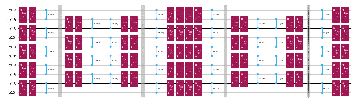
Sa halip na ipatupad nang eksakto ang time-evolution operator, maaari tayong gumamit ng Trotter decomposition upang maipatupad ang isang approximation nito. Ang paulit-ulit na paggawa ng isang partikular na order Trotter decomposition ay nagbibigay sa atin ng karagdagang pagbabawas ng error na maidudulot ng approximation. Sa sumusunod, direkta nating itatayo ang Trotter implementation sa pinakamabisang paraan para sa interaction graph ng Hamiltonian na ating isinasaalang-alang (nearest neighbor interactions lamang). Sa praktika, naglalagay tayo ng Pauli rotations na $R_{xx}$, $R_{yy}$, $R_{zz}$ na may coupling strength na $J_x,$ $J_y,$ at $J_z$ at isang parametrized na anggulo $t$, na tumutugma sa approximate na pagpapatupad ng $e^{-i (J_x XX + J_y YY + J_z ZZ) t}$. Dahil sa pagkakaiba ng depinisyon ng Pauli rotations at ng time-evolution na sinisikap nating ipatupad, kailangan nating gamitin ang parameter na $2*dt$ upang makamit ang time-evolution ng $dt$. Bukod dito, bine-reverse natin ang pagkakasunod ng mga operasyon para sa kakaibang bilang ng Trotter steps, na katumbas sa functional na paraan ngunit nagpapahintulot ng pag-synthesize ng mga katabing operasyon sa isang $SU(2)$ unitary. Nagbibigay ito ng mas mababaw na circuit kaysa sa nakuha gamit ang generic na PauliEvolutionGate() functionality.

t = Parameter("t")

# Create instruction for rotation about XX+YY-ZZ:
Rxyz_circ = QuantumCircuit(2)
Rxyz_circ.rxx(2 * JX * t, 0, 1)
Rxyz_circ.ryy(2 * JY * t, 0, 1)
Rxyz_circ.rzz(2 * JZ * t, 0, 1)
Rxyz_instr = Rxyz_circ.to_instruction(label="R J_x XX + J_y YY + J_z ZZ")

interaction_list = [
    [[i, i + 1] for i in range(0, n_qubits - 1, 2)],
    [[i, i + 1] for i in range(1, n_qubits - 1, 2)],
]  # linear chain

qr = QuantumRegister(n_qubits)
trotter_step_circ = QuantumCircuit(qr)
for i, color in enumerate(interaction_list):
    for interaction in color:
        trotter_step_circ.append(Rxyz_instr, interaction)
    if i < len(interaction_list) - 1:
        trotter_step_circ.barrier()
reverse_trotter_step_circ = trotter_step_circ.reverse_ops()

qc_evol = QuantumCircuit(qr)
for step in range(num_trotter_steps):
    if step % 2 == 0:
        qc_evol = qc_evol.compose(trotter_step_circ)
    else:
        qc_evol = qc_evol.compose(reverse_trotter_step_circ)

qc_evol.decompose().draw("mpl", fold=-1, scale=0.5)

Maghahanda tayo ng initial state muli para sa mahusay na Hadamard test na ito.

control = 0
excitation = int(n_qubits / 2) + 1
controlled_state_prep = QuantumCircuit(n_qubits + 1)
controlled_state_prep.cx(control, excitation)
controlled_state_prep.draw("mpl", fold=-1, scale=0.5)

Template circuit para sa pagkalkula ng mga matrix element ng $\tilde{S}$ at $\tilde{H}$ sa pamamagitan ng Hadamard test

Ang tanging pagkakaiba sa pagitan ng mga circuit na ginagamit sa Hadamard test ay ang phase sa time-evolution operator at ang mga observable na sinusukat. Kaya maaari tayong maghanda ng template circuit na kumakatawan sa generic na circuit para sa Hadamard test, na may mga placeholder para sa mga gate na nakasalalay sa time-evolution operator.

# Parameters for the template circuits
parameters = []
for idx in range(1, krylov_dim):
    parameters.append(dt_circ * (idx))

# Create modified hadamard test circuit
qr = QuantumRegister(n_qubits + 1)
qc = QuantumCircuit(qr)
qc.h(0)
qc.compose(controlled_state_prep, list(range(n_qubits + 1)), inplace=True)
qc.barrier()
qc.compose(qc_evol, list(range(1, n_qubits + 1)), inplace=True)
qc.barrier()
qc.x(0)
qc.compose(controlled_state_prep.inverse(), list(range(n_qubits + 1)), inplace=True)
qc.x(0)

qc.decompose().draw("mpl", fold=-1)

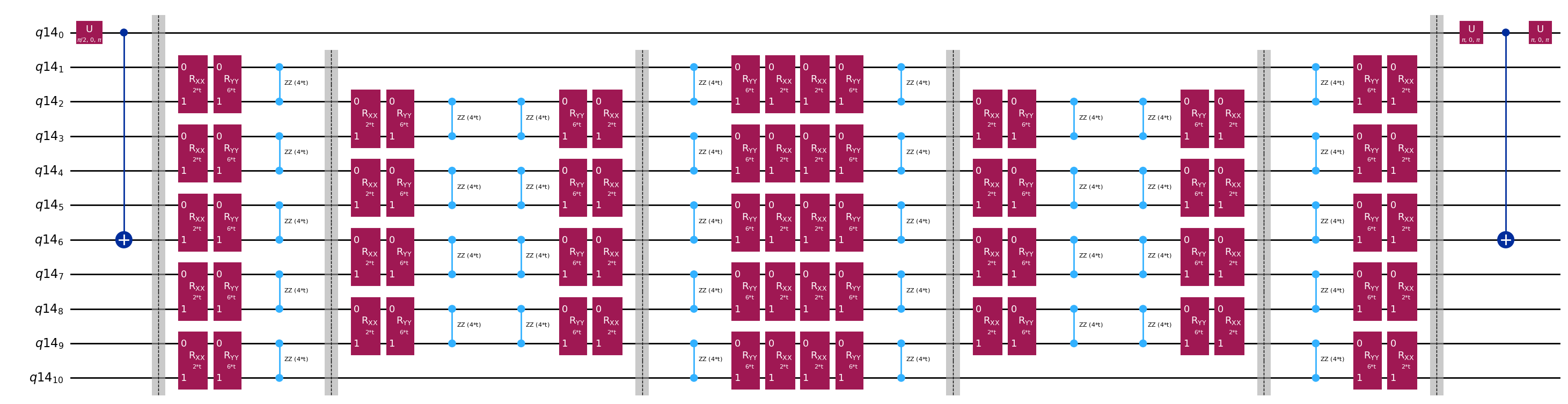
print(
    "The optimized circuit has 2Q gates depth: ",
    qc.decompose().decompose().depth(lambda x: x[0].num_qubits == 2),
)

The optimized circuit has 2Q gates depth:  50

Malaki ang pagbaba ng lalim kumpara sa orihinal na Hadamard test. Kaya-kaya na ito ng mga modernong quantum computer, kahit medyo mataas pa rin. Kailangan nating gumamit ng pinakabagong error mitigation upang makakuha ng magagamit na resulta.

Pumili ng backend kung saan tatakbo ang ating quantum Krylov calculation, para mai-transpile ang ating circuit para sa pagpapatakbo sa quantum computer na iyon.

# Use the least-busy backend or specify a quantum computer using the syntax commented out below.
service = QiskitRuntimeService()
backend = service.least_busy(operational=True, simulator=False)

# Or you may choose a specify backend and channel if necessary for your workflow.
# service = QiskitRuntimeService(channel="ibm_quantum_platform")
# backend = service.backend("ibm_fez")

I-transpile na natin ngayon ang ating mga circuit at operator.

from qiskit.transpiler.preset_passmanagers import generate_preset_pass_manager

target = backend.target
basis_gates = list(target.operation_names)
pm = generate_preset_pass_manager(
    optimization_level=3, backend=backend, basis_gates=basis_gates
)

qc_trans = pm.run(qc)

print(qc_trans.depth(lambda x: x[0].num_qubits == 2))
print(qc_trans.count_ops())
qc_trans.draw("mpl", fold=-1, idle_wires=False, scale=0.5)

36
OrderedDict([('rz', 410), ('sx', 361), ('cz', 156), ('x', 18), ('barrier', 6)])

Pagkatapos ng optimization, nabawasan pa ang two-qubit depth ng ating transpiled circuit.

4.3 Hakbang 3. Isagawa gamit ang Qiskit Runtime primitive

Gagawa tayo ngayon ng mga PUB para sa pagpapatakbo gamit ang Estimator.

# Define observables to measure for S
observable_S_real = "I" * (n_qubits) + "X"
observable_S_imag = "I" * (n_qubits) + "Y"

observable_op_real = SparsePauliOp(
    observable_S_real
)  # define a sparse pauli operator for the observable
observable_op_imag = SparsePauliOp(observable_S_imag)

layout = qc_trans.layout  # get layout of transpiled circuit
observable_op_real = observable_op_real.apply_layout(
    layout
)  # apply physical layout to the observable
observable_op_imag = observable_op_imag.apply_layout(layout)
observable_S_real = (
    observable_op_real.paulis.to_labels()
)  # get the label of the physical observable
observable_S_imag = observable_op_imag.paulis.to_labels()

observables_S = [[observable_S_real], [observable_S_imag]]

# Define observables to measure for H
# Hamiltonian terms to measure
observable_list = []
for pauli, coeff in zip(H_op.paulis, H_op.coeffs):
    # print(pauli)
    observable_H_real = pauli[::-1].to_label() + "X"
    observable_H_imag = pauli[::-1].to_label() + "Y"
    observable_list.append([observable_H_real])
    observable_list.append([observable_H_imag])

layout = qc_trans.layout

observable_trans_list = []
for observable in observable_list:
    observable_op = SparsePauliOp(observable)
    observable_op = observable_op.apply_layout(layout)
    observable_trans_list.append([observable_op.paulis.to_labels()])

observables_H = observable_trans_list

# Define a sweep over parameter values
params = np.vstack(parameters).T

# Estimate the expectation value for all combinations of
# observables and parameter values, where the pub result will have
# shape (# observables, # parameter values).
pub = (qc_trans, observables_S + observables_H, params)

Ang mga circuit para sa $t=0$ ay maaaring kalkulahin nang klasikal. Gagawin natin ito bago lumipat sa $t\neq 0$ na kaso gamit ang quantum computer.

from qiskit.quantum_info import StabilizerState, Pauli

qc_cliff = qc.assign_parameters({t: 0})

# Get expectation values from experiment
S_expval_real = StabilizerState(qc_cliff).expectation_value(
    Pauli("I" * (n_qubits) + "X")
)
S_expval_imag = StabilizerState(qc_cliff).expectation_value(
    Pauli("I" * (n_qubits) + "Y")
)

# Get expectation values
S_expval = S_expval_real + 1j * S_expval_imag

H_expval = 0
for obs_idx, (pauli, coeff) in enumerate(zip(H_op.paulis, H_op.coeffs)):
    # Get expectation values from experiment
    expval_real = StabilizerState(qc_cliff).expectation_value(
        Pauli(pauli[::-1].to_label() + "X")
    )
    expval_imag = StabilizerState(qc_cliff).expectation_value(
        Pauli(pauli[::-1].to_label() + "Y")
    )
    expval = expval_real + 1j * expval_imag

    # Fill-in matrix elements
    H_expval += coeff * expval

print(H_expval)

(10+0j)

Kahit nabawasan natin ang ating gate depth nang ilang order of magnitude gamit ang mahusay na Hadamard test, ang lalim ay sapat pa rin upang mangailangan ng pinakabagong error mitigation. Sa ibaba, tinutukoy natin ang mga katangian ng mitigation na gagamitin. Lahat ng pamamaraan ay mahalaga, ngunit sulit na banggitin nang partikular ang probabilistic error amplification (PEA). Ang makapangyarihang teknikong ito ay may malaking quantum overhead. Ang kalkulasyong ginagawa dito ay maaaring tumagal ng 20 minuto o higit pa upang tumakbo sa isang tunay na quantum computer. Maaari mong baguhin ang mga parameter sa ibaba upang dagdagan o bawasan ang katumpakan at kaugnay na overhead. Ang mga default na setting sa ibaba ay nagbibigay ng mataas na katumpakan na mga resulta.

# Experiment options
num_randomizations = 300
num_randomizations_learning = 20
max_batch_circuits = 20
shots_per_randomization = 100
learning_pair_depths = [0, 4, 24]
noise_factors = [1, 1.3, 1.6]

# Base option formatting
options = {
    # Builtin resilience settings for ZNE
    "resilience": {
        "measure_mitigation": True,
        "zne_mitigation": True,
        "zne": {"noise_factors": noise_factors},
        # TREX noise learning configuration
        "measure_noise_learning": {
            "num_randomizations": num_randomizations_learning,
            "shots_per_randomization": shots_per_randomization,
        },
        # PEA noise model configuration
        "layer_noise_learning": {
            "max_layers_to_learn": 10,
            "layer_pair_depths": learning_pair_depths,
            "shots_per_randomization": shots_per_randomization,
            "num_randomizations": num_randomizations_learning,
        },
    },
    # Randomization configuration
    "twirling": {
        "num_randomizations": num_randomizations,
        "shots_per_randomization": shots_per_randomization,
        "strategy": "all",
    },
    # Experimental settings for PEA method
    "experimental": {
        # # Just in case, disable any further qiskit transpilation not related to twirling / DD
        # "skip_transpilation": True,
        # Execution configuration
        "execution": {
            "max_pubs_per_batch_job": max_batch_circuits,
            "fast_parametric_update": True,
        },
        # Error Mitigation configuration
        "resilience": {
            # ZNE Configuration
            "zne": {
                "amplifier": "pea",
                "return_all_extrapolated": True,
                "return_unextrapolated": True,
                "extrapolated_noise_factors": [0] + noise_factors,
            }
        },
    },
}

Sa wakas, isasagawa natin ang mga circuit para sa $\tilde{S}$ at $\tilde{H}$ gamit ang Estimator.

# This job required 17 minutes of QPU time to run on a Heron r2 processor. This is only an estimate. Your execution time may vary.

with Batch(backend=backend) as batch:
    # Estimator
    estimator = Estimator(mode=batch, options=options)

    job = estimator.run([pub], precision=1)

4.4 Hakbang 4. Post-process at suriin ang mga resulta

Ang nakuha natin mula sa quantum computer ay ang mga indibidwal na matrix element ng $\tilde{S}$ at ang mga commuting Pauli group na bumubuo ng mga matrix element ng $\tilde{H}$. Kailangang pagsamahin ang mga term na ito upang mabawi ang ating mga matrix, para masulbarang natin ang generalized eigenvalue problem.

# Store the outputs as 'results'.
results = job.result()[0]

Kalkulahin ang Effective Hamiltonian at Overlap matrices

Una, kalkulahin ang phase na naipon ng estado ng $\vert 0 \rangle$ sa panahon ng walang kontrol na time evolution

prefactors = [
    np.exp(-1j * sum([c for p, c in H_op.to_list() if "Z" in p]) * i * dt)
    for i in range(1, krylov_dim)
]

Kapag mayroon na tayong mga resulta ng circuit execution, maaari na tayong mag-post-process ng data upang kalkulahin ang mga matrix element ng $S$

# Assemble S, the overlap matrix of dimension D:
S_first_row = np.zeros(krylov_dim, dtype=complex)
S_first_row[0] = 1 + 0j

# Add in ancilla-only measurements:
for i in range(krylov_dim - 1):
    # Get expectation values from experiment
    expval_real = results.data.evs[0][0][i]  # automatic extrapolated evs if ZNE is used
    expval_imag = results.data.evs[1][0][i]  # automatic extrapolated evs if ZNE is used

    # Get expectation values
    expval = expval_real + 1j * expval_imag
    S_first_row[i + 1] += prefactors[i] * expval

S_first_row_list = S_first_row.tolist()  # for saving purposes

S_circ = np.zeros((krylov_dim, krylov_dim), dtype=complex)

# Distribute entries from first row across matrix:
for i, j in it.product(range(krylov_dim), repeat=2):
    if i >= j:
        S_circ[j, i] = S_first_row[i - j]
    else:
        S_circ[j, i] = np.conj(S_first_row[j - i])

from sympy import Matrix

Matrix(S_circ)

$$\displaystyle \left[\begin{matrix}1.0 & 0.149322296177984 - 0.283023058106896 i & 0.185815978760175 - 0.0910521940394691 i & 0.0940509850777074 - 0.094154537369141 i\\0.149322296177984 + 0.283023058106896 i & 1.0 & 0.149322296177984 - 0.283023058106896 i & 0.185815978760175 - 0.0910521940394691 i\\0.185815978760175 + 0.0910521940394691 i & 0.149322296177984 + 0.283023058106896 i & 1.0 & 0.149322296177984 - 0.283023058106896 i\\0.0940509850777074 + 0.094154537369141 i & 0.185815978760175 + 0.0910521940394691 i & 0.149322296177984 + 0.283023058106896 i & 1.0\end{matrix}\right]$$

At ang mga matrix element ng $\tilde{H}$

import itertools

# Assemble S, the overlap matrix of dimension D:
H_first_row = np.zeros(krylov_dim, dtype=complex)
H_first_row[0] = H_expval

for obs_idx, (pauli, coeff) in enumerate(zip(H_op.paulis, H_op.coeffs)):
    # Add in ancilla-only measurements:
    for i in range(krylov_dim - 1):
        # Get expectation values from experiment
        expval_real = results.data.evs[2 + 2 * obs_idx][0][
            i
        ]  # automatic extrapolated evs if ZNE is used
        expval_imag = results.data.evs[2 + 2 * obs_idx + 1][0][
            i
        ]  # automatic extrapolated evs if ZNE is used

        # Get expectation values
        expval = expval_real + 1j * expval_imag
        H_first_row[i + 1] += prefactors[i] * coeff * expval

H_first_row_list = H_first_row.tolist()

H_eff_circ = np.zeros((krylov_dim, krylov_dim), dtype=complex)

# Distribute entries from first row across matrix:
for i, j in itertools.product(range(krylov_dim), repeat=2):
    if i >= j:
        H_eff_circ[j, i] = H_first_row[i - j]
    else:
        H_eff_circ[j, i] = np.conj(H_first_row[j - i])

from sympy import Matrix

Matrix(H_eff_circ)

$$\displaystyle \left[\begin{matrix}10.0 & -3.02044405310714 - 2.80721615865252 i & 0.496487054782717 + 0.188101957039621 i & 1.0770511571923 + 0.104340737159455 i\\-3.02044405310714 + 2.80721615865252 i & 10.0 & -3.02044405310714 - 2.80721615865252 i & 0.496487054782717 + 0.188101957039621 i\\0.496487054782717 - 0.188101957039621 i & -3.02044405310714 + 2.80721615865252 i & 10.0 & -3.02044405310714 - 2.80721615865252 i\\1.0770511571923 - 0.104340737159455 i & 0.496487054782717 - 0.188101957039621 i & -3.02044405310714 + 2.80721615865252 i & 10.0\end{matrix}\right]$$

Sa wakas, maaari na nating sulbarang ang generalized eigenvalue problem para sa $\tilde{H}$:

$\tilde{H} \vec{c} = c S \vec{c}$

at makakuha ng pagtatantya ng ground state energy na $c_{min}$

gnd_en_circ_est_list = []
for d in range(1, krylov_dim + 1):
    # Solve generalized eigenvalue problem
    gnd_en_circ_est = solve_regularized_gen_eig(
        H_eff_circ[:d, :d], S_circ[:d, :d], threshold=1e-1
    )
    gnd_en_circ_est_list.append(gnd_en_circ_est)
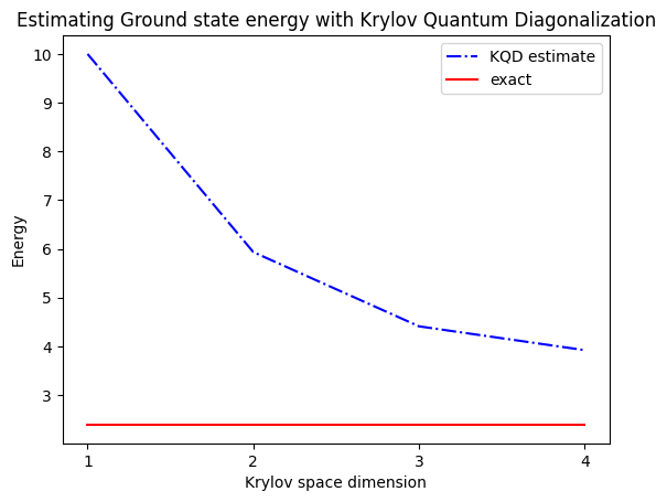
    print("The estimated ground state energy is: ", gnd_en_circ_est)

The estimated ground state energy is:  10.0
The estimated ground state energy is:  5.933953916292923
The estimated ground state energy is:  4.4101773995740645
The estimated ground state energy is:  3.921288588521255

Para sa single-particle sector, maaari tayong mahusay na kalkulahin ang ground state ng sector ng Hamiltonian na ito nang klasikal

gs_en = single_particle_gs(H_op, n_qubits)

n_sys_qubits 10
n_exc 1 , subspace dimension 11
single particle ground state energy:  2.391547869638771

len(H_op)

27

plt.plot(
    range(1, krylov_dim + 1),
    gnd_en_circ_est_list,
    color="blue",
    linestyle="-.",
    label="KQD estimate",
)
plt.plot(
    range(1, krylov_dim + 1),
    [gs_en] * krylov_dim,
    color="red",
    linestyle="-",
    label="exact",
)
plt.xticks(range(1, krylov_dim + 1), range(1, krylov_dim + 1))
plt.legend()
plt.xlabel("Krylov space dimension")
plt.ylabel("Energy")
plt.title("Estimating Ground state energy with Krylov Quantum Diagonalization")
plt.show()

5. Talakayan at pagpapalawak

Para ibuod, nagsisimula tayo sa isang reference state, pagkatapos ay ini-evolve ito sa iba't ibang tagal ng panahon para mabuo ang unitary Krylov subspace. Ini-project natin ang ating Hamiltonian sa subspace na iyon. Tinatantya rin natin ang mga overlap ng mga subspace vector. Sa wakas, kinakalkulahin natin ang mas maliit na dimensional na generalized eigenvalue problem sa pamamagitan ng klasikal na paraan.

Ikumpara natin kung ano ang nagtatakda ng computational costs kapag ginamit ang Krylov technique sa klasikal at quantum na paraan. Walang perpektong katumbas sa pagitan ng klasikal at quantum na mga approach para sa lahat ng hakbang. Kinokolekta ng talahanayang ito ang ilang scaling ng iba't ibang hakbang para sa pagsasaalang-alang.

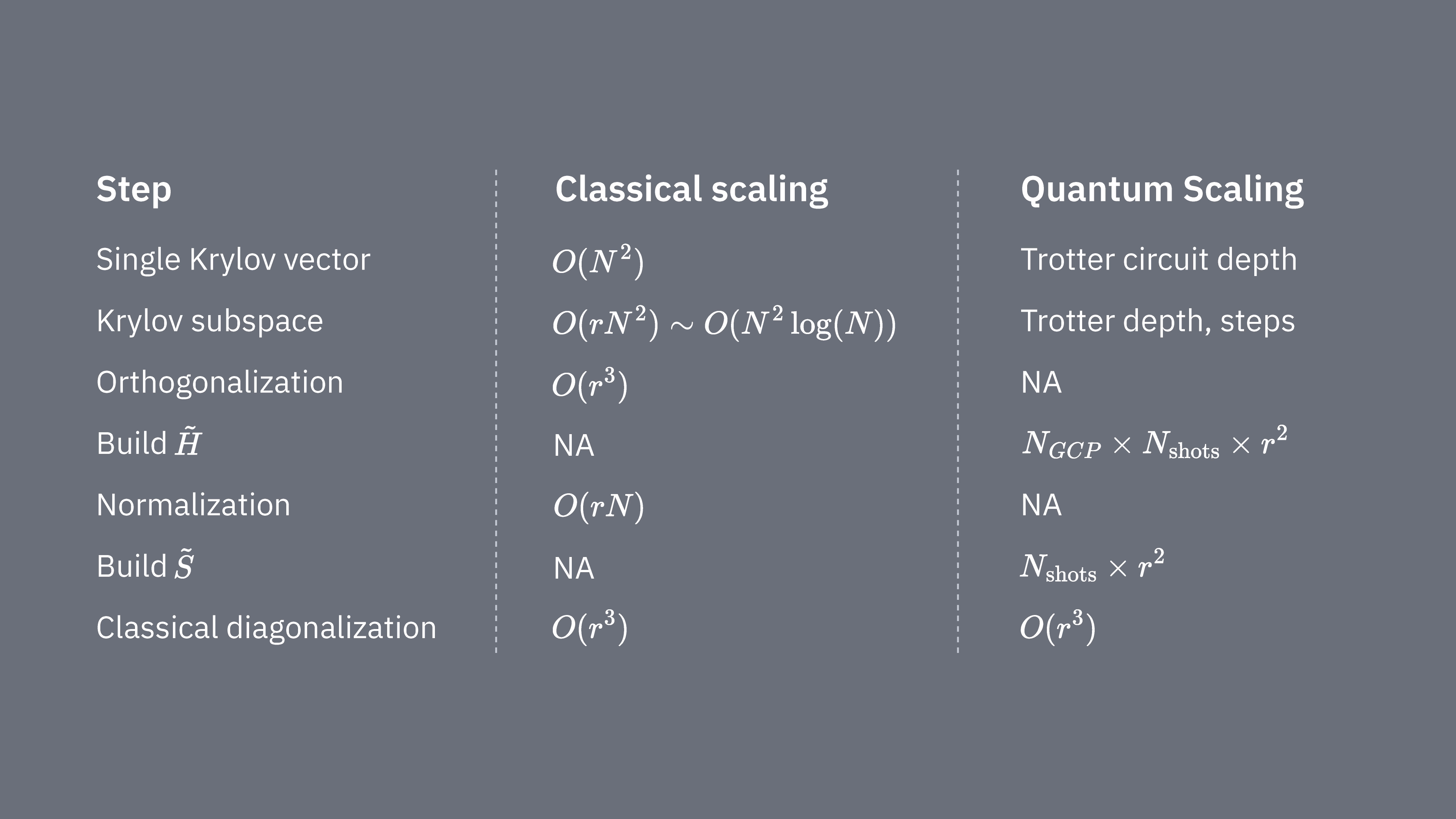
Alalahanin na ang mga Hamiltonian ay karaniwang may mga termino na hindi maaaring sabay na masukat (dahil hindi sila nag-commute sa isa't isa). Inuuri natin ang mga termino sa Hamiltonian sa mga grupo ng mga commuting Pauli operator na maaaring sabay na masukat, at maaaring kailangan natin ng maraming ganitong grupo para masaklaw ang lahat ng mga termino na hindi nag-commute sa isa't isa. Para mabuo ang $\tilde{H}$ sa isang quantum computer, kailangan ng hiwalay na mga sukat para sa bawat grupo ng mga commuting Pauli string sa Hamiltonian, at ang bawat isa sa mga ito ay nangangailangan ng maraming shots. Kailangan itong gawin para sa $r^2$ na iba't ibang matrix element, na naaayon sa $r^2$ na kombinasyon ng iba't ibang time evolution factor. Minsan may mga paraan para mabawasan ito, ngunit sa magaspang na pagtrato na ito, ang oras na kinakailangan para dito ay nag-sscale tulad ng $N_\text{shots}\times N_\text{GCP} \times r^2.$ Ang mga elemento ng $S$ ay kailangang matantya, na nag-sscale tulad ng $O(N_\text{shots}\times r^2)$. Sa wakas, ang paglutas ng generalized eigenvalue problem sa projected space, sa pamamagitan ng klasikal na paraan, ay nangangailangan ng $O(r^3).$

Nakikita natin na ang quantum Krylov diagonalization ay maaaring maging kapaki-pakinabang sa mga kaso kung saan ang bilang ng mga commuting Pauli group sa Hamiltonian ay medyo maliit. Ang mga scaling dependency na ito ay nagmumungkahi ng ilang application kung saan ang Krylov method ay maaaring maging kapaki-pakinabang, at ang iba naman ay malamang na hindi. Ang ilang Hamiltonian ay may mataas na complexity kapag na-map sa mga qubit, na kinasasangkutan ng maraming non-commuting Pauli string na hindi madaling mahati sa iilang commuting group. Ito ay madalas na totoo sa mga problema sa quantum chemistry, halimbawa. Ang complexity na ito ay nagdudulot ng dalawang pangunahing hamon para sa mga near-term quantum computer:

• Ang pagtantya ng bawat elemento ng $\tilde{H}$ ay nagiging computationally expensive dahil sa malaking bilang ng mga termino.
• Ang mga kinakailangang Trotter circuit ay nagiging napakalalim para maging praktikal.

Ang parehong punto sa itaas ay magiging hindi gaanong problema kapag naabot ng mga quantum computer ang fault-tolerance, ngunit dapat itong isaalang-alang sa kasalukuyan. Kahit ang mga sistema na may "mas simpleng" mapping kaysa sa mga nasa quantum chemistry ay maaaring makaranas ng parehong hadlang, kung ang mga Hamiltonian ay may masyadong maraming non-commuting na termino. Ang Krylov method ay pinaka-kapaki-pakinabang kung saan ang Hamiltonian ay maaaring hatiin sa medyo iilang commuting Pauli group, at kung saan ang $H$ ay madaling ipatupad sa mga Trotter circuit. Ang parehong kondisyon na ito ay natutugunan, halimbawa, para sa maraming lattice model na may interes sa physics. Ang KQD ay lalong kapaki-pakinabang kung napakakaunting alam tungkol sa ground state. Ito ay nagmumula sa likas na mga garantiya ng convergence nito at sa kakayahan nitong gamitin sa mga sitwasyon kung saan ang mga alternatibong paraan ay hindi angkop dahil sa kakulangan ng kaalaman tungkol sa ground state.

Kahit na ang KQD ay isang makapangyarihang kasangkapan, ang mga nakakapagod na aspeto ng protocol, lalo na ang pagtantya ng bawat elemento ng projected Hamiltonian at ang overlap ng mga Krylov state, ay nagbibigay ng pagkakataon para sa pagpapabuti. Ang isang alternatibong approach ay kinabibilangan ng paggamit ng mga Krylov method kasabay ng mga sampling-based na paraan, na siyang paksa ng susunod na aralin.

6. Mga Apendiks

Apendiks I: Krylov subspace mula sa real time-evolution

Ang unitary Krylov space ay tinukoy bilang

$$\mathcal{K}_U(H, |\psi\rangle) = \text{span}\left\{ |\psi\rangle, e^{-iH\,dt} |\psi\rangle, \dots, e^{-irH\,dt} |\psi\rangle \right\}$$

para sa ilang timestep na $dt$ na matatukoy natin sa ibaba. Pansamantalang ipagpalagay na ang $r$ ay pantay: pagkatapos ay tukuyin natin ang $d=r/2$. Pansinin na kapag ini-project natin ang Hamiltonian sa Krylov space sa itaas, ito ay hindi matukoy mula sa Krylov space

$$\mathcal{K}_U(H, |\psi\rangle) = \text{span}\left\{ e^{i\,d\,H\,dt}|\psi\rangle, e^{i(d-1)H\,dt} |\psi\rangle, \dots, e^{-i(d-1)H\,dt} |\psi\rangle, e^{-i\,d\,H\,dt} |\psi\rangle \right\},$$

iyon ay, kung saan ang lahat ng time-evolution ay inilipat ng $d$ na timestep paataas. Ang dahilan kung bakit hindi ito matukoy ay dahil ang mga matrix element

$$\tilde{H}_{j,k} = \langle\psi|e^{i\,j\,H\,dt}He^{-i\,k\,H\,dt}|\psi\rangle=\langle\psi|He^{i(j-k)H\,dt}|\psi\rangle$$

ay hindi nagbabago sa ilalim ng pangkalahatang paglilipat ng evolution time, dahil ang mga time-evolution ay nag-commute sa Hamiltonian. Para sa kaganapan na $r$ ay gansal, maaari nating gamitin ang pagsusuri para sa $r-1$.

Nais nating ipakita na sa loob ng Krylov space na ito, may garantiya na mayroon isang low-energy state. Ginagawa natin ito sa pamamagitan ng sumusunod na resulta, na hango mula sa Theorem 3.1 sa [3]:

Pahayag 1: mayroong isang function na $f$ na para sa mga enerhiya $E$ sa spectral range ng Hamiltonian (iyon ay, sa pagitan ng ground state energy at ng maximum energy)...

1. $f(E_0)=1$
2. $|f(E)|\le2\left(1 + \delta\right)^{-d}$ para sa lahat ng halaga ng $E$ na nasa $\ge\delta$ na layo mula sa $E_0$, iyon ay, ito ay exponentially suppressed
3. $f(E)$ ay isang linear combination ng $e^{ijE\,dt}$ para sa $j=-d,-d+1,...,d-1,d$

Nagbibigay tayo ng patunay sa ibaba, ngunit maaari itong laktawan maliban kung nais ng isa na maunawaan ang buong, mahigpit na argumento. Sa ngayon ay nakatuon tayo sa mga implikasyon ng pahayag sa itaas. Sa pamamagitan ng katangian 3 sa itaas, makikita natin na ang shifted Krylov space sa itaas ay naglalaman ng estado na $f(H)|\psi\rangle$. Ito ang ating low-energy state. Para maunawaan kung bakit, isulat ang $|\psi\rangle$ sa energy eigenbasis:

$$|\psi\rangle = \sum_{k=0}^{N}\gamma_k|E_k\rangle,$$

kung saan ang $|E_k\rangle$ ay ang kth energy eigenstate at ang $\gamma_k$ ay ang amplitude nito sa initial state na $|\psi\rangle$. Ipinahayag sa mga terminong ito, ang $f(H)|\psi\rangle$ ay ibinibigay ng

$$f(H)|\psi\rangle = \sum_{k=0}^{N}\gamma_kf(E_k)|E_k\rangle,$$

gamit ang katotohanan na maaari nating palitan ang $H$ ng $E_k$ kapag kumikilos ito sa eigenstate na $|E_k\rangle$. Ang energy error ng estado na ito ay samakatuwid

$$\text{energy error} = \frac{\langle\psi|f(H)(H-E_0)f(H)|\psi\rangle}{\langle\psi|f(H)^2|\psi\rangle}$$ $$= \frac{\sum_{k=0}^{N}|\gamma_k|^2f(E_k)^2(E_k-E_0)}{\sum_{k=0}^{N}|\gamma_k|^2f(E_k)^2}.$$

Para gawing upper bound na mas madaling maunawaan, unang hinahati natin ang sum sa numerator sa mga termino na may $E_k-E_0\le\delta$ at mga termino na may $E_k-E_0>\delta$:

$$\text{energy error} = \frac{\sum_{E_k\le E_0+\delta}|\gamma_k|^2f(E_k)^2(E_k-E_0)}{\sum_{k=0}^{N}|\gamma_k|^2f(E_k)^2} + \frac{\sum_{E_k> E_0+\delta}|\gamma_k|^2f(E_k)^2(E_k-E_0)}{\sum_{k=0}^{N}|\gamma_k|^2f(E_k)^2}.$$

Maaari nating i-upper bound ang unang termino ng $\delta$,

$$\frac{\sum_{E_k\le E_0+\delta}|\gamma_k|^2f(E_k)^2(E_k-E_0)}{\sum_{k=0}^{N}|\gamma_k|^2f(E_k)^2} < \frac{\delta\sum_{E_k\le E_0+\delta}|\gamma_k|^2f(E_k)^2}{\sum_{k=0}^{N}|\gamma_k|^2f(E_k)^2} \le \delta,$$

kung saan ang unang hakbang ay sumusunod dahil ang $E_k-E_0\le\delta$ para sa bawat $E_k$ sa sum, at ang ikalawang hakbang ay sumusunod dahil ang sum sa numerator ay isang subset ng sum sa denominator. Para sa ikalawang termino, una ay ina-lower bound natin ang denominator ng $|\gamma_0|^2$, dahil $f(E_0)^2=1$: pagtitipon-tipunin ang lahat ng ito, nagbibigay ito ng

$$\text{energy error} \le \delta + \frac{1}{|\gamma_0|^2}\sum_{E_k>E_0+\delta}|\gamma_k|^2f(E_k)^2(E_k-E_0).$$

Para pasimplehin ang natitira, pansinin na para sa lahat ng $E_k$ na ito, ayon sa kahulugan ng $f$ alam natin na $f(E_k)^2 \le 4\left(1 + \delta\right)^{-2d}$. Dagdag pa rito, ang pag-upper bound ng $E_k-E_0<2\|H\|$ at ang pag-upper bound ng $\sum_{E_k>E_0+\delta}|\gamma_k|^2<1$ ay nagbibigay ng

$$\text{energy error} \le \delta + \frac{8}{|\gamma_0|^2}\|H\|\left(1 + \delta\right)^{-2d}.$$

Naaangkop ito para sa anumang $\delta>0$, kaya kung itutumbas natin ang $\delta$ sa ating layunin na error, ang error bound sa itaas ay exponentially nagco-converge patungo roon kasabay ng Krylov dimension na $2d=r$. Pansinin din na kung $\delta<E_1-E_0$ ang $\delta$ na termino ay ganap na nawawala sa bound sa itaas.

Para kumpletuhin ang argumento, una ay pinapanatili natin na ang nasa itaas ay ang energy error lamang ng partikular na estado na $f(H)|\psi\rangle$, at hindi ang energy error ng pinakamababang energy state sa Krylov space. Gayunpaman, ayon sa (Rayleigh-Ritz) variational principle, ang energy error ng pinakamababang energy state sa Krylov space ay na-upper bound ng energy error ng anumang estado sa Krylov space, kaya ang nasa itaas ay upper bound din sa energy error ng pinakamababang energy state, iyon ay, ang output ng Krylov quantum diagonalization algorithm.

Ang katulad na pagsusuri tulad ng nasa itaas ay maaaring isagawa na kasama rin ang noise at ang thresholding procedure na tinalakay sa notebook. Tingnan ang [2] at [4] para sa pagsusuring ito.

Apendiks II: patunay ng Pahayag 1

Ang sumusunod ay karamihang hango mula sa [3], Theorem 3.1: hayaan ang $0 < a < b$ at hayaan ang $\Pi^*_d$ na maging espasyo ng mga residual polynomial (mga polynomial na ang halaga sa 0 ay 1) ng degree na hindi hihigit sa $d$. Ang solusyon sa

$$\beta(a, b, d) = \min_{p \in \Pi^*_d} \max_{x \in [a, b]} |p(x)| \quad$$

ay

$$p^*(x) = \frac{T_d\left(\frac{b + a - 2x}{b - a}\right)}{T_d\left(\frac{b + a}{b - a}\right)}, \quad$$

at ang kaukulang minimal na halaga ay

$$\beta(a, b, d) = T_d^{-1}\left(\frac{b + a}{b - a}\right).$$

Nais nating i-convert ito sa isang function na maaaring natural na ipahayag sa mga tuntunin ng complex exponential, dahil ang mga ito ang mga real time-evolution na bumubuo ng quantum Krylov space. Para magawa ito, maginhawa na ipakilala ang sumusunod na transformation ng mga enerhiya sa loob ng spectral range ng Hamiltonian patungo sa mga numero sa hanay na $[0,1]$: tukuyin ang

$$g(E) = \frac{1-\cos\big((E-E_0)dt\big)}{2},$$

kung saan ang $dt$ ay isang timestep na nagbibigay ng $-\pi < E_0dt < E_\text{max}dt < \pi$. Pansinin na $g(E_0)=0$ at ang $g(E)$ ay lumalaki habang lumalayo ang $E$ mula sa $E_0$.

Ngayon gamit ang polynomial na $p^*(x)$ na may mga parameter na a, b, d na itinakda sa $a = g(E_0 + \delta)$, $b = 1$, at d = int(r/2), tinutukoy natin ang function:

$$f(E) = p^* \left( g(E) \right) = \frac{T_d\left(1 + 2\frac{\cos\big((E-E_0)dt\big) - \cos\big(\delta\,dt\big)}{1 +\cos\big(\delta\,dt\big)}\right)}{T_d\left(1 + 2\frac{1-\cos\big(\delta\,dt\big)}{1 + \cos\big(\delta\,dt\big)}\right)}$$

kung saan ang $E_0$ ay ang ground state energy. Makikita natin sa pamamagitan ng pagpasok ng $\cos(x)=\frac{e^{ix}+e^{-ix}}{2}$ na ang $f(E)$ ay isang trigonometric polynomial ng degree na $d$, iyon ay, isang linear combination ng $e^{ijE\,dt}$ para sa $j=-d,-d+1,...,d-1,d$. Bukod pa rito, mula sa kahulugan ng $p^*(x)$ sa itaas mayroon tayong $f(E_0)=p(0)=1$ at para sa anumang $E$ sa spectral range na nagbibigay ng $\vert E-E_0 \vert > \delta$ mayroon tayong

$$|f(E)| \le \beta(a, b, d) = T_d^{-1}\left(1 + 2\frac{1-\cos\big(\delta\,dt\big)}{1 + \cos\big(\delta\,dt\big)}\right)$$ $$\leq 2\left(1 + \delta\right)^{-d} = 2\left(1 + \delta\right)^{-\lfloor k/2\rfloor}.$$

Mga Sanggunian:

[1] https://arxiv.org/abs/2407.14431

[2] https://arxiv.org/abs/1811.09025

[3] https://people.math.ethz.ch/~mhg/pub/biksm.pdf

[4] https://academic.oup.com/book/36426

[5] https://en.wikipedia.org/wiki/Krylov_subspace

[6] Krylov Subspace Methods: Principles and Analysis, Jörg Liesen, Zdenek Strakos https://academic.oup.com/book/36426

[7] Iterative Methods for Sparse Linear Systems" ni Yousef Saad

[8] "MINRES-QLP: A Krylov Subspace Method for Indefinite or Singular Symmetric Systems" ni Sou-Cheng Choi, Christopher Paige, at Michael Saunders (https://epubs.siam.org/doi/10.1137/100787921)

[9] Ethan N. Epperly, Lin Lin, at Yuji Nakatsukasa. "A theory of quantum subspace diagonalization". SIAM Journal on Matrix Analysis and Applications 43, 1263–1290 (2022).