Gumamit ng iba't ibang Lp-norm para sa Pauli term truncation

Tandaan: Bago basahin ang gabay na ito, basahin muna ang gabay na Truncate Pauli terms, na naglalarawan ng pag-truncate ng mga low-weight na Pauli term na built-in sa method na backpropagate batay sa isang tinukoy na TruncationErrorBudget. Sa gabay na ito, malalaman mo ang tungkol sa keyword argument ng backpropagate na p_norm, na magagamit para palitan ang Lp-norm na ginagamit sa pagtantya ng error na dulot ng mga na-truncate na Pauli term.

Gumawa ng halimbawang circuit

Ginagamit ng gabay na ito ang parehong halimbawang circuit tulad ng sa gabay na Truncate Pauli terms:

# Added by doQumentation — installs the packages this notebook needs if they are missing
import importlib.util

_needed = {"matplotlib": "matplotlib", "qiskit": "qiskit", "qiskit_addon_obp": "qiskit-addon-obp", "qiskit_addon_utils": "qiskit-addon-utils", "rustworkx": "rustworkx"}
_missing = [pip for module, pip in _needed.items()
            if importlib.util.find_spec(module) is None]
# One at a time, so a package that fails to install does not block the others
for _pip in _missing:
    %pip install -q {_pip}
if not _missing:
    print("\u2713 All required packages are installed")

import rustworkx.generators
from qiskit.synthesis import LieTrotter
from qiskit_addon_utils.problem_generators import (
    PauliOrderStrategy,
    generate_time_evolution_circuit,
    generate_xyz_hamiltonian,
)
from qiskit_addon_utils.slicing import combine_slices, slice_by_gate_types

# Generate a linear chain of 10 qubits
num_qubits = 10
linear_chain = rustworkx.generators.path_graph(num_qubits)

# Use an arbitrary XY model
hamiltonian = generate_xyz_hamiltonian(
    linear_chain,
    coupling_constants=(0.05, 0.02, 0.0),
    ext_magnetic_field=(0.02, 0.08, 0.0),
    pauli_order_strategy=PauliOrderStrategy.InteractionThenColor,
)
# Evolve for some time
circuit = generate_time_evolution_circuit(
    hamiltonian, synthesis=LieTrotter(reps=3), time=2.0
)
# slice the circuit by gate type
slices = slice_by_gate_types(circuit)

# For visualization purposes only, recombine the slices with barriers between them and draw the resulting circuit
combine_slices(slices, include_barriers=True).draw("mpl", fold=50, scale=0.6)

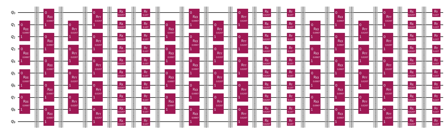
Mag-define ng observable para sa kabuuang magnetization:

from qiskit.quantum_info import SparsePauliOp

obs = SparsePauliOp.from_sparse_list(
    [("Z", [i], 1.0) for i in range(num_qubits)], num_qubits=num_qubits
)

Bilang reference, kalkulahin ang eksaktong expectation value:

from qiskit.primitives import StatevectorEstimator

estimator = StatevectorEstimator()
job = estimator.run([(circuit, obs)])
res = job.result()
exact_exp = res[0].data.evs
print(exact_exp)

9.318197859862146

Gamitin ang L1 norm

Bilang default, at gaya ng nakita mo na sa gabay na Truncate Pauli terms, p_norm=1, na ang ibig sabihin ay tinatantya ang error bilang:

$$|\langle\psi|\Delta|\psi\rangle| \leq \sum_{P\in\mathcal{T}} |c_P|$$

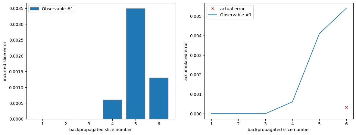
kung saan ang $\psi$ ay ang quantum state, ang $\Delta$ ay ang totoong pagkakaiba ng eksakto at na-truncate na observable (na hindi alam), ang $\mathcal{T}$ ay ang set ng mga Pauli term na na-truncate, at ang $c_P$ ay ang coefficient ng Pauli term. Ang inequality na ito ay isang mahigpit ngunit napaluwag na upper bound sa karamihan ng mga sitwasyon. Sa gabay na ito, bina-backpropagate ang anim na slice ng halimbawang circuit, gamit ang pare-parehong error kada slice na 0.001. Ang halagang ito ay dapat unawain bilang budget sa loob ng ibinigay na p_norm.

from qiskit_addon_obp.utils.truncating import setup_budget

l1_truncation_error_budget = setup_budget(max_error_per_slice=0.001, p_norm=1)
print(l1_truncation_error_budget)

TruncationErrorBudget(per_slice_budget=[0.001], max_error_total=inf, p_norm=1)

from qiskit_addon_obp import backpropagate

max_slices = 6
l1_bp_obs, l1_remaining_slices, l1_metadata = backpropagate(
    obs,
    slices[-max_slices:],
    truncation_error_budget=l1_truncation_error_budget,
)
l1_reduced_circuit = combine_slices(
    slices[:-max_slices] + l1_remaining_slices
)
print(
    f"Backpropagated {max_slices - len(l1_remaining_slices)} circuit slices."
)
print(
    f"New observable contains {len(l1_bp_obs)} terms and {len(l1_bp_obs.group_commuting(qubit_wise=True))} commuting groups."
)

Backpropagated 6 circuit slices.
New observable contains 116 terms and 10 commuting groups.

Ngayon ay maaari na nating kalkulahin ang expectation value ng na-backpropagate na observable, pati na ang error kumpara sa eksaktong reference:

estimator = StatevectorEstimator()
job = estimator.run([(l1_reduced_circuit, l1_bp_obs)])
res = job.result()
l1_exp = res[0].data.evs
l1_error = exact_exp - l1_exp
print(l1_exp, l1_error)

9.317869899338842 0.00032796052330397174

Panghuli, maaari nating i-plot ang error na naipon sa backpropagation ng bawat slice, pati na ang naipon na kabuuang error. Ang naipon na error ay ang kabuuan ng mga error ng bawat slice. Makikita natin na ang naipon na error ay isang napaluwag na upper bound sa totoong error.

from matplotlib import pyplot as plt
from qiskit_addon_obp.utils.visualization import (
    plot_accumulated_error,
    plot_slice_errors,
)

fig, axes = plt.subplots(1, 2, figsize=(14, 5))
axes[1].plot([6], [l1_error], "x", color="red", label="actual error")
plot_slice_errors(l1_metadata, axes[0])
plot_accumulated_error(l1_metadata, axes[1])

Gamitin ang L2 norm

Maaaring sabihin na ang L2 norm ay mas mahusay na pagtantya ng nangyaring error kaysa sa L1 norm. Dahil maaari nating ipalagay na ang quantum state na $|\psi\rangle$ ay hinango mula sa isang Haar random ensemble, kung saan ang nangyaring error ay sumusunod sa isang distribusyon na may nawawalang mean at isang variance na maaaring tantiyahing i-bound ng L2 norm:

$$|\langle\psi|\Delta|\psi\rangle| \lesssim \left( \sum_{P\in\mathcal{T}} |c_P|^2 \right)^{1/2}$$

Bagama't hindi mahigpit ang bound, malalabag lang ito sa mga pathological na kaso. Muli nating bina-backpropagate ang anim na slice ng halimbawang circuit, gamit ang pinakamataas na error kada slice na 0.001 (sa pagkakataong ito, binibigyang-kahulugan sa L2 norm).

l2_truncation_error_budget = setup_budget(max_error_per_slice=0.001, p_norm=2)
print(l2_truncation_error_budget)

TruncationErrorBudget(per_slice_budget=[0.001], max_error_total=inf, p_norm=2)

max_slices = 6
l2_bp_obs, l2_remaining_slices, l2_metadata = backpropagate(
    obs,
    slices[-max_slices:],
    truncation_error_budget=l2_truncation_error_budget,
)
l2_reduced_circuit = combine_slices(
    slices[:-max_slices] + l2_remaining_slices
)
print(
    f"Backpropagated {max_slices - len(l2_remaining_slices)} circuit slices."
)
print(
    f"New observable contains {len(l2_bp_obs)} terms and {len(l2_bp_obs.group_commuting(qubit_wise=True))} commuting groups."
)

Backpropagated 6 circuit slices.
New observable contains 84 terms and 6 commuting groups.

Muli, kinakalkula natin ang expectation value ng na-backpropagate na observable at ang error kumpara sa eksaktong reference:

estimator = StatevectorEstimator()
job = estimator.run([(l2_reduced_circuit, l2_bp_obs)])
res = job.result()
l2_exp = res[0].data.evs
l2_error = exact_exp - l2_exp
print(l2_exp, l2_error)

9.317829770853422 0.00036808900872387085

Ang pag-plot ng mga error kada slice at ng naipon na error ay nagbibigay ng kahawig na larawan tulad ng dati.

fig, axes = plt.subplots(1, 2, figsize=(14, 5))
axes[1].plot([6], [l2_error], "x", color="red", label="actual error")
plot_slice_errors(l2_metadata, axes[0])
plot_accumulated_error(l2_metadata, axes[1])

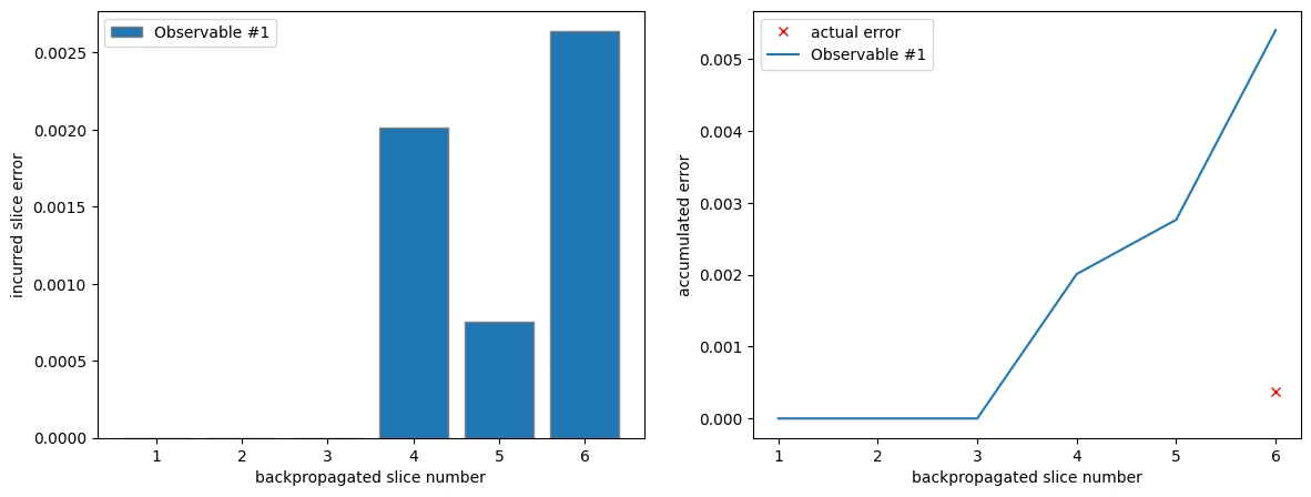
Tandaan na ang naipon na error ay muling kabuuan ng mga error ng bawat slice. Isa pa itong napaluwag na bound dahil sa Minkowski inequality, dahil kailangan nating kalkulahin ang bound na ito nang recursive:

$$|\langle\psi|\Delta_{i}|\psi\rangle| \leq |\langle\psi|\tilde{\Delta}_{i-1}|\psi\rangle| + \left( \sum_{P\in\mathcal{T_i}} |c_P|^2 \right)^{1/2} = |\langle\psi|\tilde{\Delta}_{i}|\psi\rangle|$$

kung saan ang bagong subscript na $i$ ay nagpapahiwatig ng kasalukuyang slice iteration, kaya ang $\Delta_i$ ay ang totoong error sa backpropagation iteration na $i$, ang $\tilde{\Delta}_{i-1}$ ay ang tinantyang truncation error mula sa iteration na $i-1$, at ang $\mathcal{T}_i$ ay ang set ng mga Pauli term na na-truncate sa iteration na $i$.