Pagrepaso ng mga kaugnay na paraan ng machine learning

Sa seksyong ito, rerepasoin natin ang ilang mahahalagang termino at paraan mula sa klasikal na machine learning na makakatulong sa ating mas maunawaan ang mga workflow sa quantum machine learning. Magsisimula tayo sa ilang pangkalahatang termino, bago mag-dive nang mas malalim sa dalawang uri ng machine learning: kernel methods (lalo na sa konteksto ng support vector machine) at neural networks. Tiyak na may mga koneksyon sa pagitan ng mga pamamaraang ito, ngunit itatrato natin sila nang hiwalay dahil sa mga pagkakaiba sa quantum workflows na tinalakay dito at sa mga susunod na aralin. Ito ay isang maikling pangkalahatang-ideya lamang, at maraming detalye ang laktawan natin. Para sa mas kumpletong pangkalahatang-ideya ng machine learning, inirerekomenda namin ang mga resources tulad ng [1-3].

Mga uri ng machine learning

Sa isang simpleng kahulugan, ang machine learning ay isang koleksyon ng mga algorithm na nag-aanalisa at kumukuha ng mga hinuha mula sa mga pattern at relasyon sa data. Sa malawak na pagtingin, ang mga algorithm ng machine learning ay maaaring ikategorya sa tatlong pangunahing grupo depende sa uri ng data na kasangkot at sa paraan ng pag-aaral ng mga algorithm nang hindi tahasang pinoprograma:

1. Supervised learning: Sa supervised learning, ang data na ginagamit para sanayin ang modelo ay may label. Ang layunin ng mga algorithm na ito ay matuto ng relasyon sa pagitan ng data at ng kanilang kaukulang mga label o output at ilapat ito sa hindi pa nakikitang data. Ang mga karaniwang gawain sa klaseng ito ay classification at regression.
2. Unsupervised learning: Kumpara sa supervised learning, ang unsupervised learning ay gumagamit ng unlabeled na data para sanayin ang modelo ng machine learning. Ang layunin ng mga ganitong algorithm ay tuklasin ang mga nakatagong pattern at estruktura sa data. Ang ilang algorithm sa klaseng ito ay clustering at dimensionality reduction algorithms. Ang ilang generative models tulad ng generative adversarial networks at variational autoencoders ay maaari ring isaalang-alang sa kategoryang ito.
3. Reinforcement learning: Ang mga algorithm sa kategoryang ito ng machine learning ay tinukoy ng isang ahente na nakikipag-ugnayan sa isang kapaligiran. Ang ahente ay gumagawa ng mga aksyon at tumatanggap ng feedback mula sa kapaligiran nito sa anyo ng mga gantimpala at parusa. Sa kalaunan, sa pamamagitan ng mekanismong ito ng feedback, natututo ang ahente na gawin ang tamang hanay ng mga aksyon para magsagawa ng isang partikular na gawain.

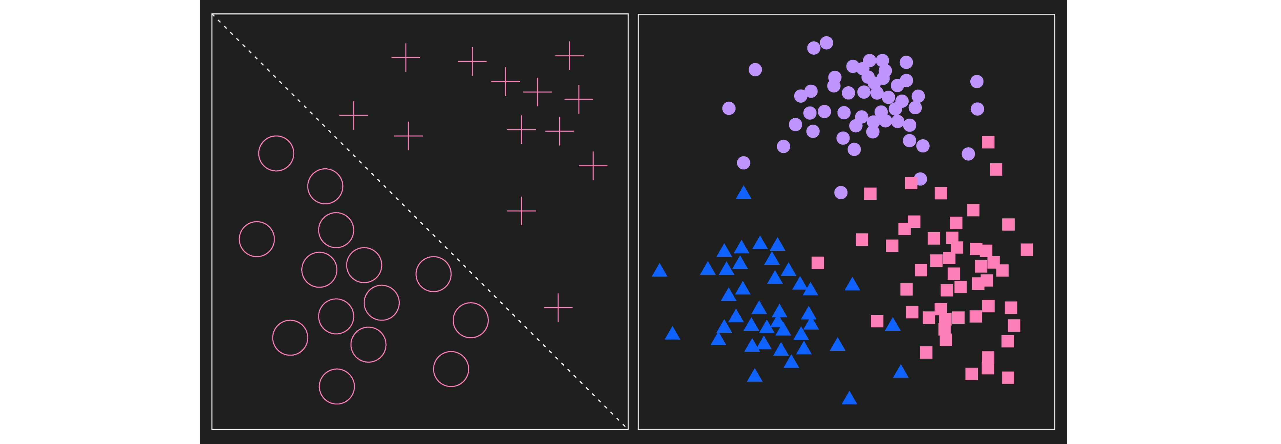
Ang kaliwang larawan ay nagpapakita ng dalawang kategorya ng labeled na data tulad ng sa supervised learning. Sa kasong ito, ang mga kategorya ay linearly separable. Ang kanang larawan ay nagpapakita ng mga cluster ng data. Sa isang unsupervised learning na gawain, ang mga data na ito ay hindi pa aalamang may label at ang algorithm ay mag-aaral ng distribusyon, marahil naghahanap ng mga cluster. Para sa layunin ng pag-visualize ng mga halimbawang cluster na maaaring matukoy ng algorithm, ang mga data point ay binigyan na ng label. Isang pangunahing pagkakaiba sa pagitan ng dalawa ay ang proseso ng supervised learning ay nagsisimula sa data na may label na at ang proseso ng unsupervised ay nagsisimula sa unlabeled na data, kahit na may label na ang data sa katapusan.

Pagpapakilala ng "quantum" sa machine learning

Maaari na tayong magsimulang tuklasin kung paano ipinapakilala ang "quantum" sa machine learning. Sa mas malawak na kategorisasyong ito, isinasaalang-alang natin ang uri ng modelo/algorithm sa processing device, pati na rin ang uri ng data na ibinibigay dito. Ang larawan sa itaas ay nagbubuod ng mga posibleng kombinasyong ito.

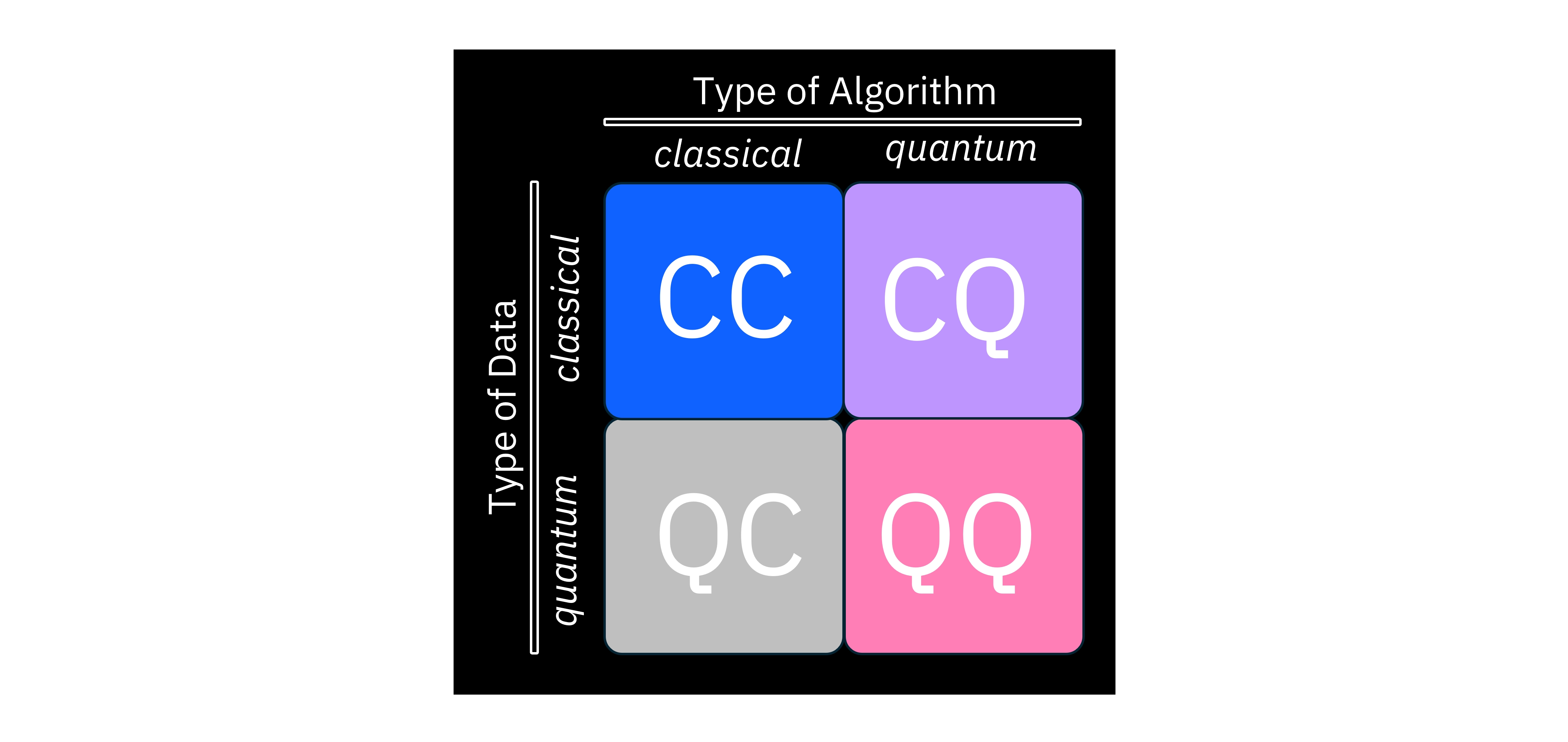
Halimbawa, ang CC ay nangangahulugang mayroon tayong klasikal na dataset — tulad ng mga larawan, tunog, o teksto na maaari nating iimbak sa mga klasikal na computer — at gumagamit din tayo ng klasikal na computer para patakbuhin ang isang machine learning algorithm. Ito mismo ang klasikal na machine learning na setting. Sa kabilang banda, ang QQ ay nangangahulugang gumagamit tayo ng quantum computer para iproseso ang quantum data. Dito, ang "quantum data" ay maaaring mangahulugan ng maraming bagay, at maaaring depende sa konteksto. Ang quantum data ay maaaring isipin bilang isang hanay ng mga resulta ng pagsukat na nakuha mula sa isang quantum device, o maaaring tumukoy sa mga estado na inihanda sa isang quantum computer ng isa pang algorithm. Sa hinaharap, maaari pa itong tumukoy sa data na nakaimbak sa QRAM (Quantum Random Access Memory), na hindi pa umiiral sa kasalukuyan. Kapag ang mga mananaliksik ay nagsasalita tungkol sa quantum machine learning, karaniwang tinutukoy nila ang CQ regime, kung saan ang dataset ay klasikal at ang processing device na nagpapatupad ng machine learning algorithm ay isang quantum computer. Sa mga sumusunod na bahagi ng kurso, magtutuon tayo sa mga ganitong algorithm.

Mga support vector machine

Ngayon ay rerepasoin natin ang isang klase ng mga algorithm na tinatawag na support vector machines mula sa pananaw ng klasikal na machine learning. Sa kalaunan ay ipapakita natin kung paano maidadagdag ang quantum computing sa algorithm na ito.

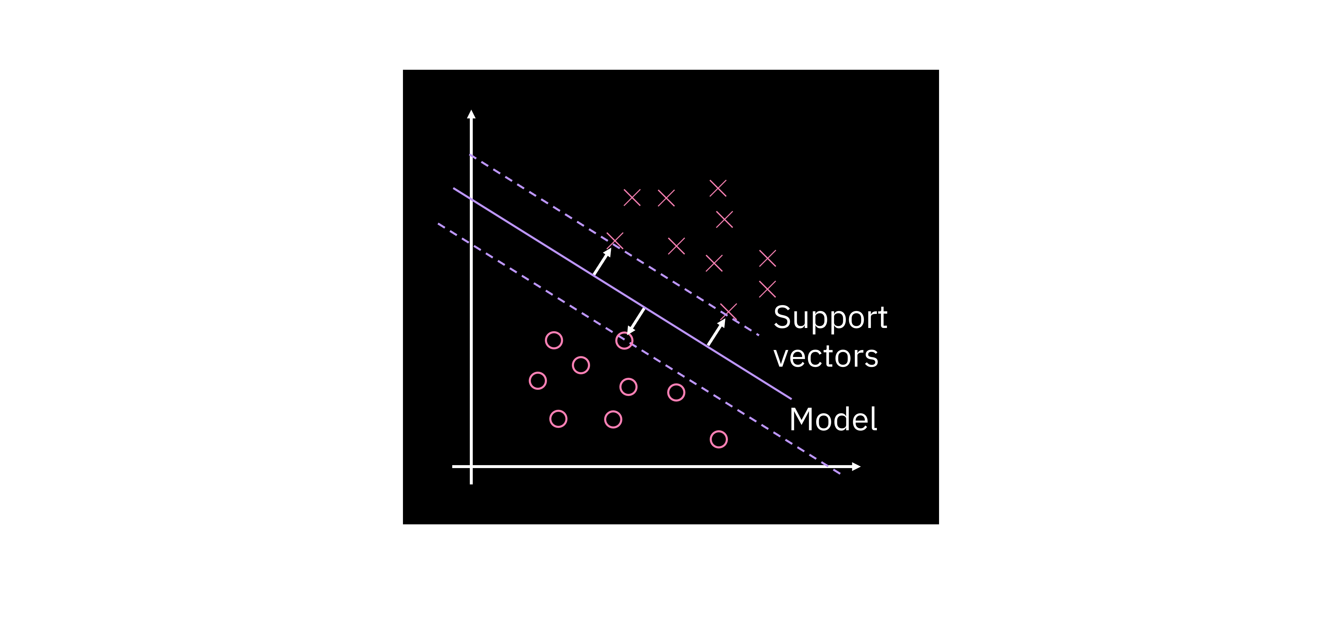
Ipagpalagay nating mayroon tayong gawain ng binary classification sa isang dataset na may two-dimensional feature space tulad ng ipinapakita sa plot. Isang bagay na maaari nating gawin para magsagawa ng classification para sa dataset na ito ay humanap ng isang linya, o sa pangkalahatan ay isang hyperplane na naghihiwalay sa dalawang klase. Sa praktis, maaari tayong makahanap ng walang katapusang maraming naghihiwalay na hyperplane, kaya ang tanong ay: Paano natin matutukoy ang pinakamainam? Ang ideya dito ay ang isang partikular na magandang decision boundary ay dapat na i-maximize ang margin, na tinutukoy bilang distansya sa pinakamalapit na mga punto sa bawat klase. Sa setting na ito, ang mga data point na may pinakamaliit na distansya sa decision boundary ay tinatawag na support vectors.

Ang isang linear decision boundary ay maaaring ilarawan sa ilang paraan; sa ilang mga paraan ang pinaka-direktang paraan ay ang ipinapakita sa $f_1$ sa ibaba. Dito, ang $\Theta$ ay ang hanay ng mga parameter na tumutukoy sa hyperplane, ang $\vec{x}$ ay ang iyong dataset, at ang $b$ ay isang constant shift. Ang $\Phi$ ay isang mapping mula sa espasyo ng mga input data point, madalas (ngunit hindi palagi) sa isang mas mataas na dimensional na espasyo. Babalikan natin ang mapping na ito sa ibaba.

Sa modelo na $f_1,$ ang $\Theta$ ay ang vector ng mga nababagong parameter na matututo ang modelo. Ito ang tinatawag nating "primal formulation". Sa pamamagitan ng ilang mathematical na manipulasyon ay maaari nating ipakita na mayroon pang ikalawang paraan na maaari nating i-formulate ang parehong problema. Tinatawag natin itong "dual formulation", na inilalarawan ng equation na $f_2$ sa ibaba. Para sa formulation na ito, kailangan nating mag-optimize sa mga alpha parameter. Ang pangunahing pagkakaiba ay ang primal formulation ay may inner product sa pagitan ng feature vector at ng mga nalalernang parameter, samantalang sa dual formulation ang inner product ay nasa pagitan ng mga feature vector. Kahit na ang dual form ay kinabibilangan ng parehong training data features at kaukulang mga label, makikita natin sa susunod na seksyon kung paano ito nagiging mas kapaki-pakinabang kaysa sa primal form.

$$f_1(\vec{x}) = \Theta^T \Phi(\vec{x})+b$$ $$f_2(\vec{x}) = \sum_{i=1}^n \alpha_i y_i \Phi^T(\vec{x}_i)\Phi(\vec{x})+b$$

Mga kernel method at kung paano makakatulong ang quantum

Ang video sa ibaba ay nagbibigay-motibasyon kung paano makakatulong ang quantum sa mga linear classifier. Ito ay mas detalyadong inilarawan sa teksto.

Paglipat sa mas mataas na dimensional na mga espasyo

Sa subseksyong ito at sa sumusunod, ang talakayan ay nakatuon sa mga mapping sa mas mataas na dimensyon. Ang punto dito ay ipaliwanag ang "kernel trick" sa konteksto ng mga mapping sa pagitan ng mga espasyo, at sa gayon ay itakda ang entablado para sa kung ano ang quantum kernel. Ang punto ay hindi na ang mas mataas na dimensyon sa quantum wave functions ay malulutas ng lahat ng ating mga problema. Tulad ng nabanggit sa panimula, ang klasikal na Gaussian feature maps ay walang katapusang dimensional na. Ang dimensionality ng mga feature ng data ay mahalaga, ngunit ang mga mataas na dimensional na quantum states ay hindi sapat para sa pagpapabuti sa mga klasikal na paraan.

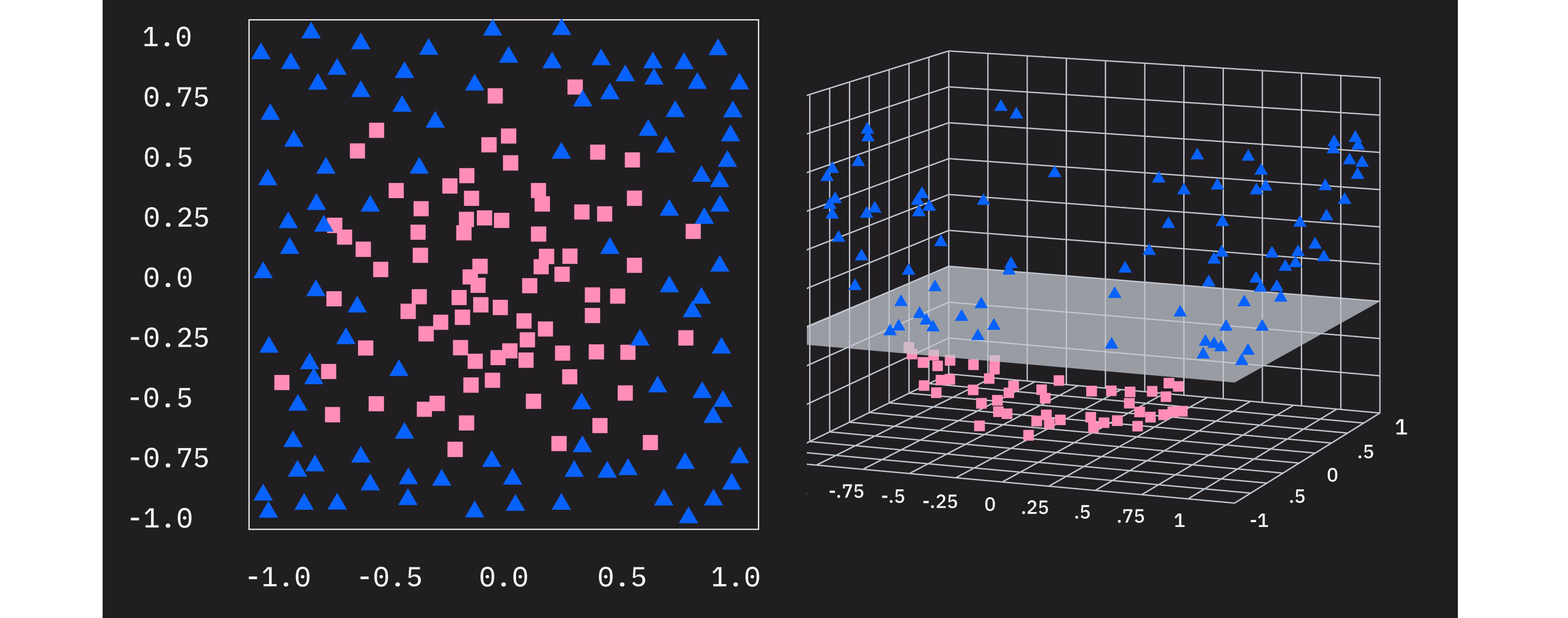
Sa graphical na paraan, madali nating makikita kung paano natin maaaring i-generalize ang SVM approach sa mga kaso kung saan ang orihinal na data ay hindi linearly separable, kapag may tamang mapping sa mas mataas na dimensyon. Tingnan ang two-dimensional na data sa kaliwa, makikita natin na walang linear decision boundary na makakapaghiwalay sa dalawang klase. Gayunpaman, maaari tayong isaalang-alang ang pagdaragdag ng ikatlong feature sa ating feature space. Kung ang bagong feature na ito ay — halimbawa — ang distansya sa pinagmulan ng nakaraang dalawang feature na $x_1$ at $x_2$, kung gayon ang data ay magiging linearly separable. Nangangahulugan din ito na maaari na nating patakbuhin nang matagumpay ang support vector machine algorithm sa mas mataas na dimensional na feature space na ito.

Tinutukoy din natin itong "feature mapping" bilang $\Phi$. Ang feature map ay madalas na nagma-map mula sa espasyo ng input data patungo sa mas mataas na dimensyon, tulad ng ipinapakita dito, ngunit may mga modelo at algorithm na gumagamit ng mga mapping sa mas mababang dimensyon. Ang mapping sa mas mataas na dimensyon ay isang madaling kaso lamang para ma-visualize at maunawaan.

$$\vec{x} = \begin{pmatrix}x_1 \\ x_2 \end{pmatrix}$$ $$\vec{\Phi}(\vec{x}) = \begin{pmatrix}x_1 \\ x_2 \\ {x_1}^2+{x_2}^2\end{pmatrix}$$

Ang ilang feature map ay maaaring mag-map sa napakataas na dimensional na mga espasyo. Sa mga ganitong kaso, ang mataas na dimensionality ay nagpapagaling ng mga inner product na mas mahal sa computational. Babalikan natin ang puntong iyon sa ibaba.

Bakit kapaki-pakinabang ang dual form?

Alalahanin ang primal at dual formulations ng ating linear boundary model:

$$f_1(\vec{x}) = \Theta^T \Phi(\vec{x})+b$$ $$f_2(\vec{x}) = \sum_{i=1}^n \alpha_i y_i \Phi^T(\vec{x}_i)\Phi(\vec{x})+b$$

Ngayon na alam na natin na ang paggamit ng isang feature map para makarating sa mas mataas na dimensional na espasyo ay makakapagpahintulot sa ating matagumpay na makahanap ng naghihiwalay na hyperplane, maaari nating palitan ang orihinal na feature vector na $\vec{x}$ sa mga equation ng mga feature-mapped na vector. Gayunpaman, kung gagawin natin ito sa primal formulation, makakatagpo tayo ng problema ng pagkakailangan na kalkulahin ang mga inner product sa pagitan ng mga parameter at ng isang potensyal na napakataas na dimensional na feature map. Gayunpaman, sa dual formulation, nakikita natin na ito ay pinalitan ng mga inner product sa pagitan ng mga feature-mapped na vector ng iba't ibang input.

Para sa ilang feature map, maaaring posible na isulat ang inner product ng mga feature-mapped na vector na $\vec{\Phi}^T(\vec{x}_i)\cdot \vec{\Phi}(\vec{x}_j)$ bilang isang simpleng function na $k(\vec{x}_i, \vec{x}_j)$ ng orihinal (mas mababang dimensional) na mga variable na $\vec{x}_i$ at $\vec{x}_j$. Para sa ilang pagpili ng $\Phi,$ maaari pa nating isulat ang $\vec{\Phi}^T(\vec{x}_i)\cdot \vec{\Phi}(\vec{x}_j)$ bilang isang simpleng function ng mas mababang dimensional na inner product na $\vec{x}_i^T\vec{x}_j$. Ito ay lubhang kapaki-pakinabang sa computational dahil maaari nating ma-access ang espasyo kung saan ang data ay linearly separable, ngunit nang wala ang gastos ng mga manipulasyon sa mas mataas na dimensyon. Sa katunayan, dahil ang mga feature-mapped na vector ay lilitaw lamang sa $f_2$ sa mga inner product, maaaring hindi na natin kailangan pang tahasang isagawa ang feature mapping para kalkulahin ang mga inner product. Tinatawag natin ang function na $k(\vec{x}_i, \vec{x}_j)$ na nagkakalkula ng mga inner product na "kernel function", at ang paraang ito ng pag-iwas sa pagkalkula ng feature map ay tinatawag na "kernel trick". Sa katunayan, ang mga feature-mapped na vector ay maaaring infinite dimensional pa, ngunit ang kernel ay maaari pa ring maging napaka-epektibong nako-compute.

Ang kernel function mismo ay isang function ng dalawang input data vector. Ang paglalagay ng bawat pares ng data vector sa dataset bilang mga argumento ng kernel function ay nagreresulta sa isang symmetric, positive semi-definite matrix, na tinatawag na kernel matrix:

$$k = \begin{pmatrix}k(\vec{x}_1,\vec{x}_1) & k(\vec{x}_1,\vec{x}_2) & ... \\ k(\vec{x}_2,\vec{x}_1) & k(\vec{x}_2,\vec{x}_2) & ... \\ \vdots & \vdots & \ddots\end{pmatrix}$$

Kapag nakalkula na natin ang kernel matrix, maaari nating hanapin ang mga pinakamainam na parameter ($\alpha_i$) gamit ang mga paraan tulad ng quadratic programming software o isang algorithm na tinatawag na "sequential minimal optimization". Siyempre, ipinapalagay nito na may isang mahusay na nako-compute na kernel na naaayon sa isang feature map na nagpapalit ng linearly separable sa iyong mga klase ng data. Isang kaugnay ngunit bagong approach ay ang quantum kernel estimation.

Mga quantum kernel

Ang mga quantum computer, o mga quantum state sa pangkalahatan, ay nagbibigay-daan sa isang napaka-natural na kahulugan ng "quantum kernel". Maaari nating ipaliwanag ang pag-encode ng isang input na $\vec{x}$ sa isang quantum state na $|\Phi(\vec{x})\rangle$ bilang isang feature map. Ang prosesong ito ay maaaring talagang mag-map ng data sa isang napakataas na dimensional na espasyo tulad ng karaniwan sa mga klasikal na feature map, ngunit ang dimensionality ay depende sa paraan ng encoding (tingnan ang aralin sa Data Encoding). Alalahanin na ang inner product ng dalawang quantum state na $\langle \psi | \phi \rangle$ ay may kaugnayan sa probabilidad ng pagsukat sa estado na $|\phi\rangle$ kapag nasa estado na $|\psi\rangle$. Maaari nating tantiyahin ang inner product ng dalawang na-map na data point na $\vec{\Phi}(\vec{x}_i)$ at $\vec{\Phi}(\vec{x}_j)$ sa pamamagitan ng paggawa ng sapat na maraming pagsukat ng resultang circuit.

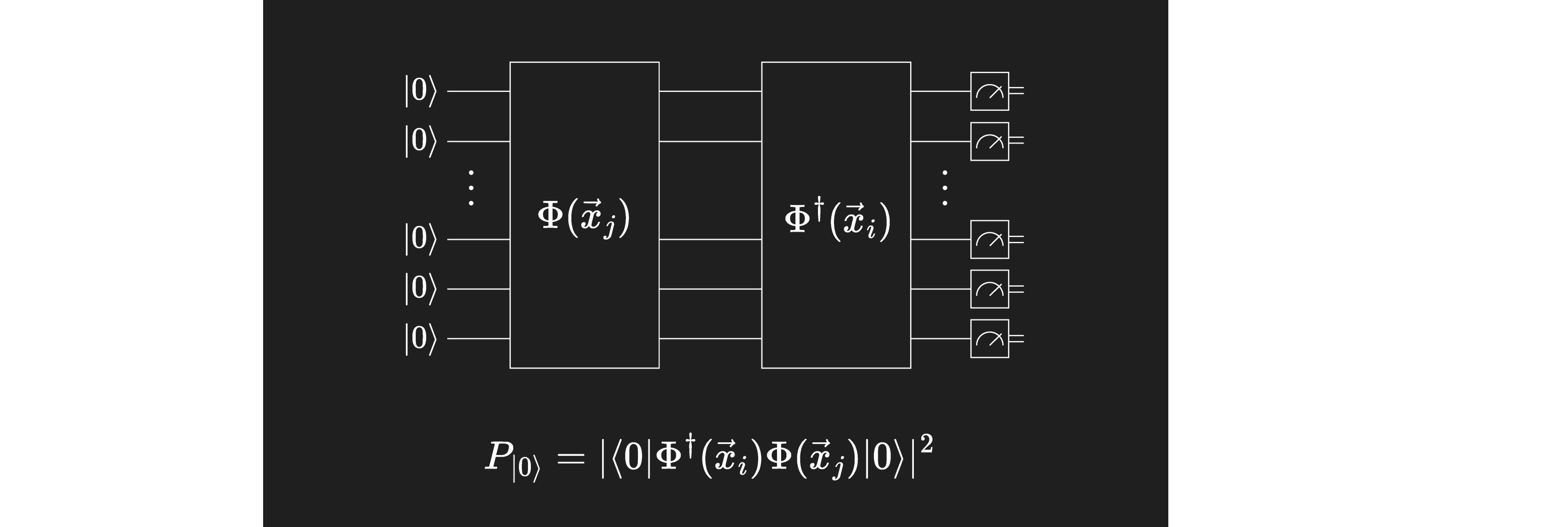
Tulad ng makikita natin sa kalaunan sa kurso, maaari tayong gumamit ng mga pagsukat sa isang quantum circuit tulad ng ipinapakita sa itaas para tantiyahin ang isang kernel, at maaari nating patakbuhin ang SVM optimization nang klasikal sa kernel matrix para matuto ng mga nababagong parameter.

Mga variational quantum classifier at neural network

Isa pang near-term quantum machine learning algorithm ay tinatawag na "variational quantum circuits" (VQCs). Kapag ang mga circuit na ito ay ginagamit sa isang gawain ng classification, maaaring makita mo ang parehong acronym na ginagamit para tumukoy sa "variational quantum classifiers" (VQCs din). Ang mga ito ay madalas na gumagamit ng mga estruktura na katulad ng klasikal na neural networks (NNs); at sa mga kasong iyon ay makikita mo silang inilarawan bilang quantum neural networks (QNNs). Mahalaga na maunawaan na ang mga VQC ay mas pangkalahatan at hindi kailangang sumunod sa isang NN na estruktura, ngunit nagsisimula tayo sa analohiya sa mga NN para malinawan ang papel na maaaring gampanan ng quantum sa mga umiiral na machine learning workflow. Tatalakayin natin ang mga generalisasyon. Nagsisimula tayo sa pamamagitan ng pagrepaso ng klasikal na neural networks.

Ang video sa ibaba ay nagbibigay ng maikling pagrepaso ng mga neural network, at kung saan sila nagtatagpo sa mga variational quantum circuit. Ito ay mas naipaliwanag sa teksto.

Ang neural network ay isang computational model na maluwag na inspirado ng estruktura at function ng mga neuron sa isang utak. Ang mga neuron na ito, na mga node na nakikita natin sa larawan, ay nakaayos sa mga layer, at konektado sa pamamagitan ng mga weight.

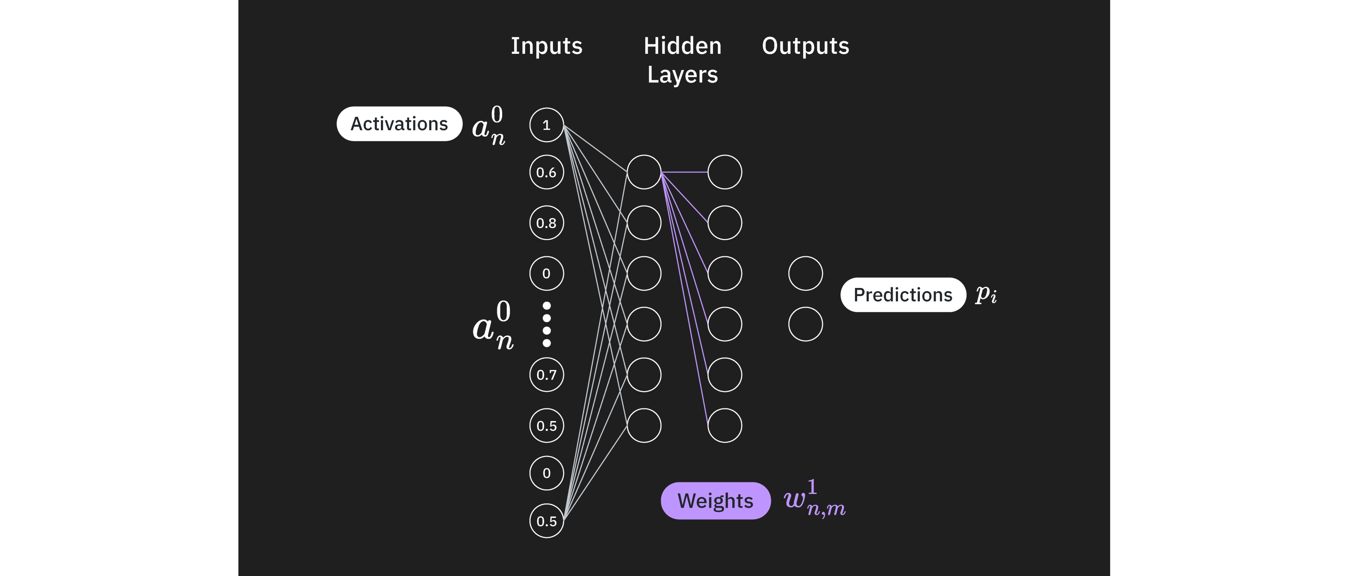
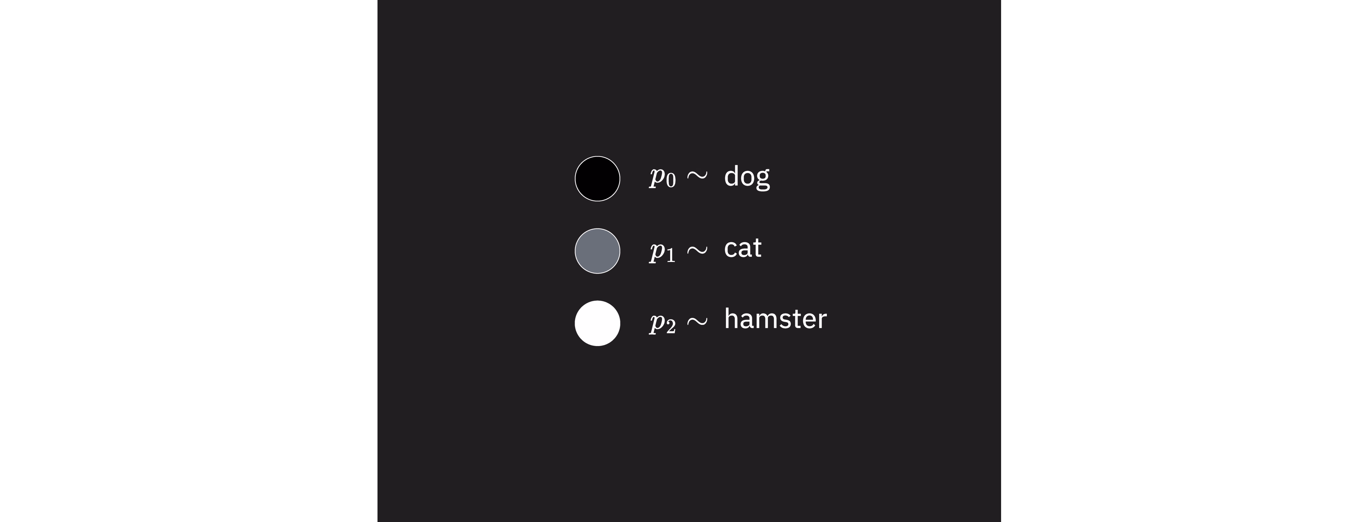
Ang unang layer ay ang input layer, at ang mga activation na $a_n^0$ ng mga neuron sa layer na ito ay direktang pinapasok mula sa data na $\vec{x}$ na susuriin (tulad ng shading ng mga indibidwal na pixel sa isang larawan, halimbawa). Ang huling layer ay isang output layer na naglalarawan ng kategorisasyon (tulad ng pag-classify ng isang larawan na may 90% tsansang ito ay isang aso, at 10% tsansang ito ay isang pusa, para manatili sa halimbawa ng larawan).

Ang mga neuron sa bawat layer ay nagpoproseso ng mga signal na tinatanggap nila mula sa nakaraang layer at ipinapadala ang mga ito sa susunod sa pamamagitan ng mga weight, $w_i$ (ang mga koneksyon sa diagram). Kung tutuunan natin ang isa sa mga neuron na ito, mayroon tayong building block ng isang neural network, na tinatawag na "perceptron". Sa mathematical na paraan, ang isang perceptron ay tumatanggap ng isang input vector na $\vec{x}$, at kinakalkula ang inner product nito sa isang trainable weight vector kasama ang ilang bias. At napakahalaga, ang perceptron ay nag-aaplay ng isang non-linear activation function ($\sigma$) sa ibabaw ng komputasyong ito. Ang mga non-linear activation function na ito ay kritikal para sa mahusay na kapangyarihang nagpapahayag ng mga neural network. Isa pang paraan para isipin ito ay, kung wala tayong non-linearity sa pagitan ng mga layer, kung gayon maaari nating isulat ang buong neural network bilang isang malaking matrix multiplication. Ito ay magreresulta lamang sa isang linear na modelo, na hindi makakayang makuha ang mga kumplikadong pattern na kaya ng malalim na neural network. Samakatuwid, ang mga nonlinear activation function ay pundamental sa mga neural network.

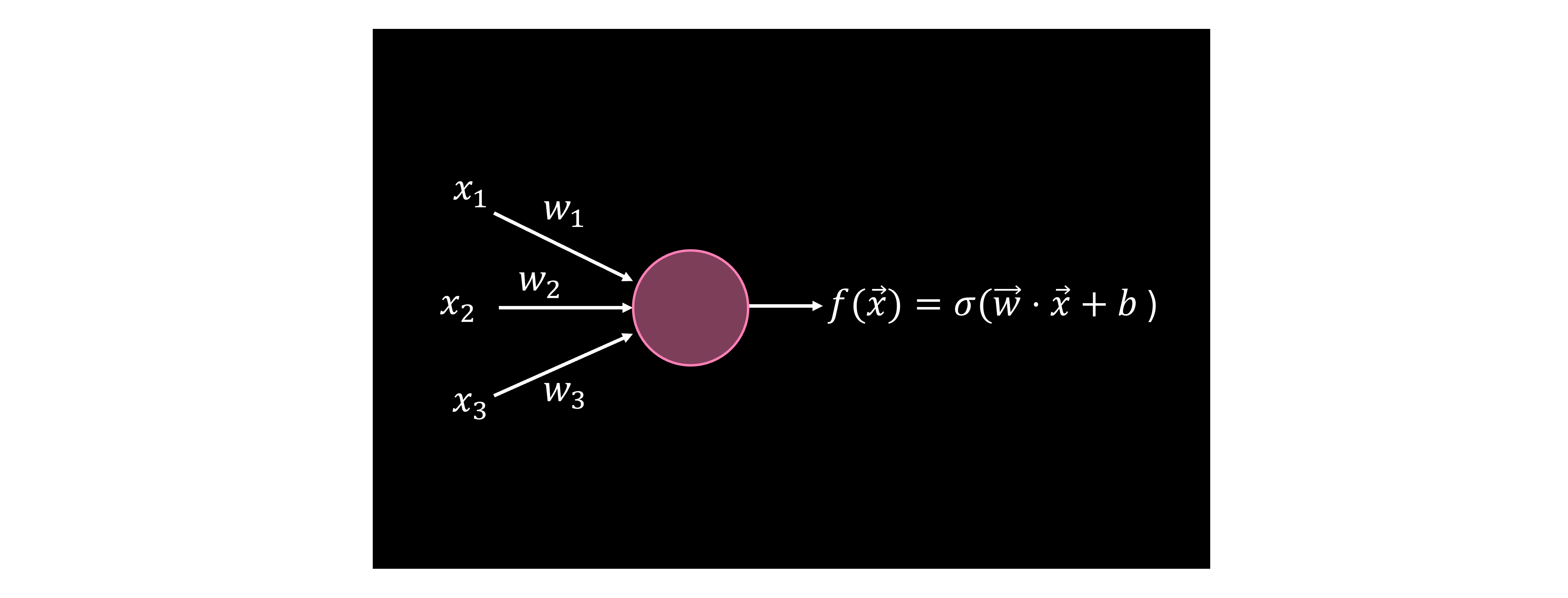
Ang mga function tulad ng

$$f(\vec{x}) = \sigma (\vec{w}\cdot \vec{x}+\vec{b})$$

ay kinakalkula sa bawat neuron gamit ang kilalang data na $\vec{x}$ at non-linear na $\sigma$ at pati na rin ang hindi kilalang mga vector ng mga weight na $\vec{w}$ at mga bias na $\vec{b}$. Sa pangkalahatan, maaaring may mga non-zero na weight sa pagitan ng lahat ng neuron ng lahat ng layer, at tatawagin natin ang mga weight mula sa layer $L$ hanggang layer $L+1$ sa pagitan ng mga neuron $m$ at $n$ bilang $w^L_{m,n}$. Katulad nito, ang bias sa $n^\text{th}$ neuron ng $L^\text{th}$ layer ay magiging $b^L_n.$ Ang mga bias dito ay walang kaugnayan sa mga $b$ mula sa talakayan ng quantum kernel.

Maaaring simulan mo ang iyong neural network na may random na hanay ng mga weight at bias, o mula sa isang kilalang makatwirang simula na configuration. Mula doon, ang ideya ay suriin kung gaano kahusay ang pag-classify ng iyong neural network at pagbutihin ito. Gumagamit tayo ng cost function para ilarawan kung paano lumalayo ang ating neural network mula sa tamang classification. Maraming paraan ng pagtukoy ng cost function. Ilalarawan natin ang isang karaniwang halimbawa dito, na kinabibilangan ng mean-squared error (MSE):

$$C(w^L_{m,n},b^L_n) = \frac{1}{N}\sum_{i=1}^{N_\text{train}}\sum_{j=1}^{N_\text{outputs}}{(v_{i,j}-p_{i,j})^2}$$

Depende sa iyong aplikasyon, maaaring nangangahulugan ito ng pagkuha ng pagkakaiba sa pagitan ng aktwal na halaga na $v_{i,j}$ ng isang larawan na $i$ mula sa training data para sa output na $j$ (halimbawa, isang halaga ng 1.0 sa output layer neuron para sa "aso" at isang 0 sa lahat ng iba pang neuron) at ang hinulaang halaga na $p_{i,j}$. I-square ang pagkakaibang iyon at i-sum sa lahat ng mga kategorya, kaya sumasaklaw ito hindi lamang kung ang tamang kategorya ay pinaka-activated, kundi pati na rin kung ang mga maling activation ay nabawasan. Pagkatapos ay i-sum natin sa lahat ng mga halimbawa sa ating training set at makakuha ng cost.

Pagkatapos ay binabago natin ang mga parameter tulad ng mga weight sa bawat layer, sa pagitan ng lahat ng mga neuron, at ang mga bias sa lahat ng neuron. Ang mga klasikal na optimization routine tulad ng gradient descent ay ginagamit para maghanap ng local minimum sa cost function.

Quantum perceptron

Para makagawa ng quantum na katapat ng perceptron, isa sa mga bagay na kailangan nating isaalang-alang ay ang kakayahang ipatupad ang non-linearity gamit ang mga quantum circuit, na siyang papel ng activation function sa mga klasikal na neural network. Ito ay dahil nang walang karagdagang mga pagsasaalang-alang, ang mga quantum circuit ay nagpapatupad lamang ng mga unitary na operasyon, na simpleng linear. May iba't ibang paraan na maaari nating gamitin para ipakilala ang non-linearity sa mga quantum circuit. Isa sa mga pangunahing paraan ay ang paggamit ng mga pagsukat bilang pinagkukunan ng non-linearity. Kasama sa iba pang mga pagsasaalang-alang ang mga pamamaraan batay sa quantum Fourier transform, mid-circuit measurements o dynamic circuits, at ang pag-trace ng mga qubit mula sa circuit.

Quantum neural network

Ang isang quantum neural network (QNN) ay gumagana sa pamamagitan ng una sa pag-encode ng input data gamit ang unitary layer na $U$ sa figure, pagkatapos ay pag-apply ng mga quantum circuit na naaayon sa mga weight sa pagitan ng mga layer ($W$ sa ibaba), at sa wakas ay isang layer ng pagsukat. Ilang mahahalagang punto tungkol dito:

• Ang pag-load ng data at mga weighting ay mga linear na operasyon.
• Ang mga pagsukat ay non-linear.
• Kaya tulad ng sa klasikal na NN, mayroon tayong parehong linear at non-linear na mga bahagi.
• Ang mga weight circuit ay may mga variational na parameter pa rin, kaya mayroon pa ring klasikal na minimization na isasagawa.

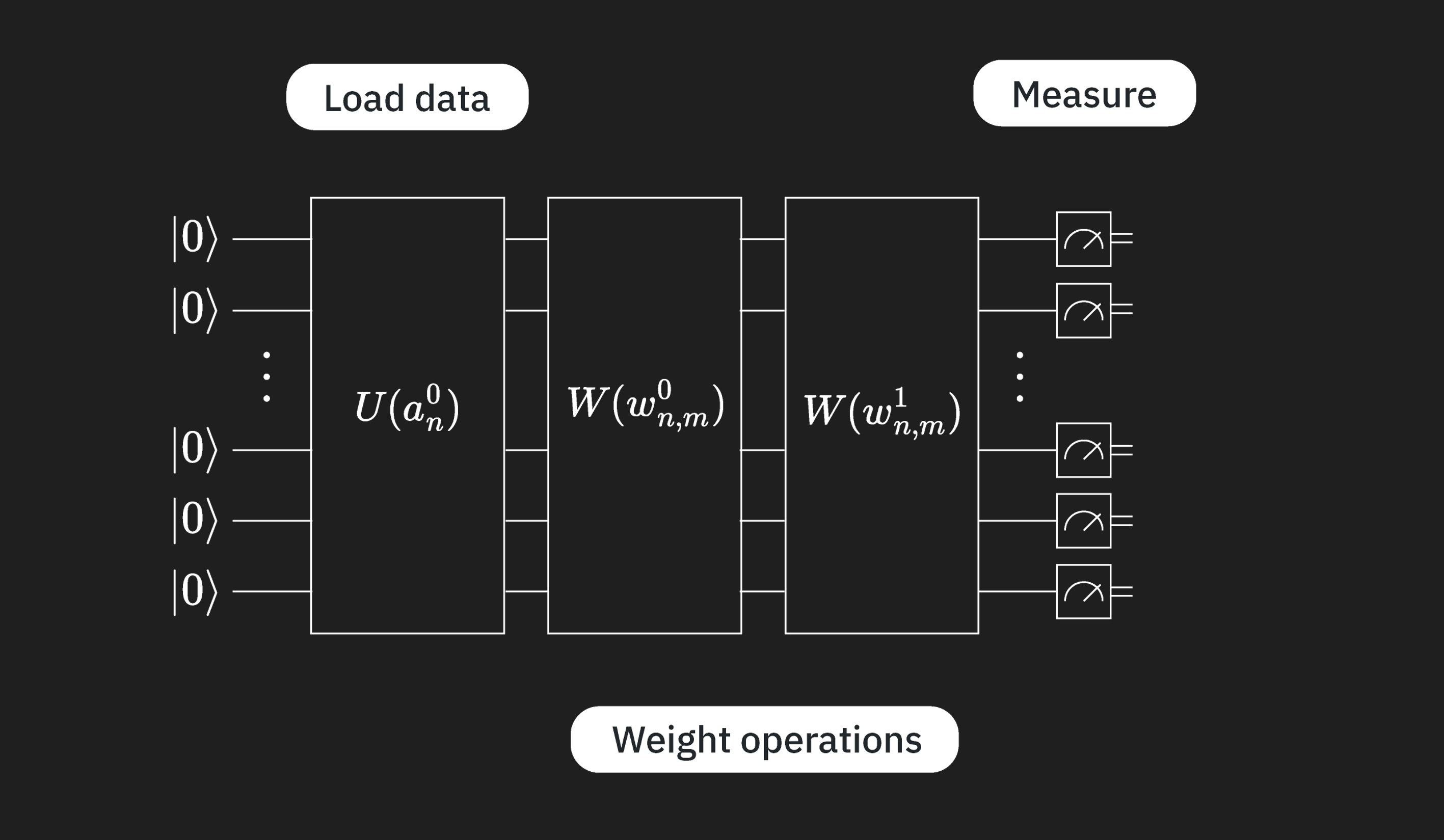
Maaari tayong gumamit ng circuit tulad ng nasa itaas para kalkulahin ang isang function $f_{QNN}(x) = \langle 0|U^{\dagger}(X)W^{\dagger}OWU(x)|0\rangle$ Pansinin na ang function na ito ay hindi sa pangkalahatan kapareho ng function na $f(x)$ na inilarawan sa klasikal na NN. Sa partikular, ang function na ito ay kinabibilangan ng potensyal na maraming layer ng maraming weight, at inilalapat sa lahat ng data na na-load sa iyong quantum circuit ng $U$.

Mga generalisasyon

Maaari na nating tingnan ang isa sa mga paraan ng pagbuo ng quantum na katapat ng isang neural network. Sa modelong ito, ang daloy ng impormasyon ay naiiba mula sa isang klasikal na feed-forward na neural network. Sa klasikal na setting, ang impormasyon ay dadaanan mula kaliwa hanggang kanan, nagsisimula sa input at nagtatapos sa output ng modelo, at sa kabaligtarang direksyon kapag gumagawa ng backpropagation para sanayin ang modelo.

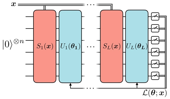
Gayunpaman, sa konstruksyon ng quantum neural network na ito, nakikita natin na ang unitary block na nag-e-encode ng data ay paulit-ulit sa pagitan ng mga variational unitary block na may mga nalalernang parameter. Ang estratehiyang ito, na tinutukoy natin bilang "data reuploading", ay sinusuportahan ng mga kawili-wiling theoretical na resulta. Sa katunayan, isang papel ni Pérez-Salinas et al. ay nagpapakita na, sa tulong ng maraming data reuploading, "ang isang qubit ay nagbibigay ng sapat na kakayahan sa computational para makagawa ng isang universal quantum classifier kapag tinulungan ng isang klasikal na subroutine." Samakatuwid, ang data reuploading ay isang teknik na maaari nating gamitin para mapahusay ang expressiveness at representational power ng modelo, na nagpapahintulot sa quantum neural network na mag-approximate ng mga kumplikadong function.

Mga sanggunian

[1] "Reinforcement Learning: An Introduction", Richard S. Sutton and Richard G. Barto, MIT Press, Second Edition, Cambridge, MA, 2018

[2] "Pattern Recognition and Machine Learning", Christopher M. Bishop, Springer, 2006

[3] "Foundations of Machine Learning", Mehryar Mohri, Afshin Rostamizadeh, and Ameet Talwalkar, MIT Press, Second Edition, 2018.