Variational Quantum Eigensolver (VQE)

Para sa modyul na ito, kailangan ng mga estudyante ng gumaganang Python environment, at ang pinakabagong bersyon ng mga sumusunod na package na naka-install:

• qiskit
• qiskit_ibm_runtime
• qiskit-aer
• qiskit.visualization
• numpy
• pylatexenc

Para i-set up at i-install ang mga package na ito, tingnan ang gabay na I-install ang Qiskit. Para makapag-run ng mga job sa tunay na quantum computer, kailangang mag-set up ng IBM Cloud account ang mga estudyante, ayon sa mga hakbang sa gabay na I-set up ang iyong IBM Cloud account.

Ang modyul na ito ay nasubok at gumamit ng humigit-kumulang 8 minuto ng QPU time. Ito ay isang pagtatantya, at ang iyong aktwal na paggamit ay maaaring mag-iba.

# Added by doQumentation — required packages for this notebook
!pip install -q matplotlib numpy qiskit qiskit-aer qiskit-ibm-runtime scipy

# Uncomment and modify this line as needed to install dependencies
#!pip install 'qiskit>=2.1.0' 'qiskit-ibm-runtime>=0.40.1' 'qiskit-aer>=0.17.0' 'numpy' 'pylatexenc'

Panimula

Mula nang mabuo ang quantum mechanical model sa unang bahagi ng ika-20 siglo, naunawaan na ng mga siyentipiko na ang mga elektron ay hindi sumusunod sa mga nakapirming landas sa paligid ng nucleus ng isang atomo, kundi nananatili sa mga rehiyon ng posibilidad na tinatawag na mga orbital. Ang mga orbital na ito ay tumutugma sa mga tiyak, diskretong antas ng enerhiya na maaaring sakupin ng mga elektron. Ang mga elektron ay natural na nananatili sa pinakamababang available na antas ng enerhiya, na kilala bilang ground state. Gayunpaman, kung ang isang elektron ay sumipsip ng sapat na enerhiya, maaari itong tumalon sa isang mas mataas na antas ng enerhiya, pumapasok sa isang excited state. Ang excited state na ito ay pansamantala, at sa kalaunan ang elektron ay babalik sa isang mas mababang antas ng enerhiya, inilalabas ang nasisipsip na enerhiya, madalas sa anyo ng liwanag. Ang pundamental na prosesong ito ng pagsipsip at paglabas ng enerhiya ay mahalaga sa pag-unawa kung paano nakikipag-ugnayan ang mga atomo at bumubuo ng mga bond.

Kapag nagtitipon ang mga atomo upang bumuo ng mga molekula, ang kanilang mga atomic orbital ay pinagsama upang bumuo ng mga molecular orbital. Ang kaayusan at mga antas ng enerhiya ng mga elektron sa loob ng mga molecular orbital na ito ang nagtatakda ng mga katangian ng nabuong molekula at ng lakas ng mga chemical bond. Halimbawa, sa pagbuo ng hydrogen molecule ($H_2$) mula sa dalawang indibidwal na hydrogen atom, ang elektron mula sa bawat atomo ay sumasakop sa mga atomic orbital. Habang papalapit ang mga atomo sa isa't isa, ang mga atomic orbital na ito ay nagtatagpo at pinagsama upang bumuo ng mga bagong molecular orbital — isa na may mas mababang enerhiya (isang bonding orbital) at isa na may mas mataas na enerhiya (isang anti-bonding orbital). Ang dalawang elektron, isa mula sa bawat hydrogen atom, ay mas gugustuhing sakupin ang mas mababang enerhiyang bonding orbital, na humahantong sa pagbuo ng isang matatag na covalent bond na nagtataglay ng $H_2$ molecule. Ang pagkakaiba ng enerhiya sa pagitan ng mga hiwalay na atomo at ng nabuong molekula, lalo na ang enerhiya ng mga elektron sa mga molecular orbital, ang nagtatakda ng katatagan at mga katangian ng bond.

Sa mga susunod na seksyon, tutuklasin natin ang prosesong ito ng pagbuo ng molekula, na nakatuon sa $H_2$ molecule. Gagamit tayo ng tunay na quantum computer, kasama ang mga klasikal na teknik ng optimization, upang mahanap ang enerhiya ng simpleng ngunit pundamental na prosesong ito. Ang eksperimentong ito ay magbibigay ng praktikal na demonstrasyon kung paano maaaring mailapat ang quantum computation sa paglutas ng mga problema sa computational chemistry, na nagbibigay ng mga pananaw tungkol sa papel ng enerhiya ng elektron.

VQE - Isang variational quantum algorithm para sa mga eigenvalue problem

Mga teknik ng approximation para sa chemistry - variational principle at ang basis set

Ang mga kontribusyon ni Erwin Schrödinger sa quantum mechanics ay hindi limitado sa pagpapakilala ng isang bagong electronic model; sa pundamental, itinatag niya ang wave mechanics sa pamamagitan ng pagbuo ng sikat na time-dependent Schrödinger equation:

$$i\hbar \frac{d}{dt}|\psi\rangle = \hat{H}|\psi\rangle$$

Dito, ang $\hat{H}$ ay ang Hamiltonian operator, na kumakatawan sa kabuuang enerhiya ng sistema, at ang $|\psi\rangle$ ay ang wave function na naglalaman ng lahat ng impormasyon tungkol sa quantum state ng sistema. (Tandaan: ang $\frac{d}{dt}$ ay ang kabuuang time derivative, at hindi natin tahasang isinasama ang energy eigenvalue na $E$ dito.)

Gayunpaman, sa maraming praktikal na aplikasyon — tulad ng pagtukoy sa mga pinapahintulutang antas ng enerhiya ng mga atomo at molekula — ginagamit namin ang time-independent Schrödinger equation (energy eigenvalue equation), na hinango mula sa time-dependent na anyo sa pamamagitan ng pag-aakala ng isang stationary state. Ang isang stationary state ay isang quantum state kung saan ang probability density ng paghanap ng isang particle sa isang naibigay na punto sa espasyo ay hindi nagbabago sa paglipas ng panahon.

$\hat{H}|\psi\rangle = E|\psi\rangle$

Sa anyo na ito, ang $E$ ay kumakatawan sa energy eigenvalue na tumutugma sa quantum state na $|\psi\rangle$. Kasama sa Hamiltonian ang iba't ibang kontribusyon ng enerhiya, tulad ng kinetic energy ng mga elektron at nuclei, ang mga attractive force sa pagitan ng mga elektron at nuclei, at ang mga repulsive force sa pagitan ng mga elektron.

Ang paglutas ng energy eigenvalue equation ay nagbibigay-daan sa atin na kalkulahin ang mga quantized na antas ng enerhiya ng mga atomic at molecular system. Gayunpaman, para sa mga molekula, mahirap ito lutasin nang eksakto dahil ang wave function na $\Psi$, na naglalarawan ng spatial distribution ng mga elektron, ay kumplikado at mataas ang dimensyon.

Bilang resulta, gumagamit ang mga siyentipiko ng mga teknik ng approximation upang makakuha ng mga praktikal at tumpak na solusyon. Sa gawaing ito, magtutuon tayo sa dalawang pangunahing pamamaraan:

1. Variational principle

   Ang pamamaraang ito ay nag-a-approximate ng wave function at ina-adjust ito upang mapalapit hangga't maaari sa target na enerhiya, kadalasan ang ground state energy ng sistema. Ang pangunahing ideya sa likod ng variational principle ay simple:

   • Kung hulaan natin ang isang wave function na $\Psi_\text{trial}$ (isang "trial function"), ang enerhiyang kinakalkula mula rito ay palaging magiging katumbas o mas mataas kaysa sa ground state energy ($E_0$) ng sistema. $E_\text{approx} = \frac{\langle \Psi_\text{trial}|\hat{H}|\Psi_\text{trial}\rangle}{\langle \Psi_\text{trial}|\Psi_\text{trial}\rangle} \geq E_0$
   • Sa pamamagitan ng pag-adjust ng mga parameter na $\theta$ sa trial function, $|\Psi_\text{trial}(\theta)\rangle$, makakakuha tayo ng mas magandang approximation ng ground state energy.
   • Ang katumpakan nito ay lubos na nakasalalay sa pagpili ng trial wave function na $\Psi_\text{trial}$. Ang isang masamang pagpili ng trial function ay maaaring humantong sa isang pagtatantya ng enerhiya na malayo sa tumpak.

2. Basis set approximation

   Ang pangalawang pamamaraan ng approximation ay dumarating sa yugto ng pagbuo ng wave function — ang basis set approach. Sa quantum chemistry, halos imposibleng lutasin nang eksakto ang Schrödinger equation para sa mga molekula. Sa halip, ini-approximate natin ang kumplikado, multi-electron wave function sa pamamagitan ng pagbuo nito mula sa mas simpleng, paunang natukoy na mga mathematical function. Ang isang basis set ay mahalagang isang koleksyon ng mga kilalang mathematical function na ito, karaniwang nakasentro sa mga atomo sa molekula, na ginagamit bilang mga building block upang kumatawan sa hugis at gawi ng mga elektron sa sistema. Isipin ito na parang sinusubukang muling likhain ang isang detalyadong eskultura gamit lamang isang koleksyon ng mga karaniwang LEGO brick — habang mas maraming uri at sukat ng brick ang mayroon ka (mas malaki ang basis set), mas tumpak mong ma-a-approximate ang orihinal na hugis.

   Ang mga basis function na ito ay madalas na inspirado ng mga analytical na solusyon para sa mga simpleng sistema tulad ng hydrogen atom, na kumukuha ng mga anyo tulad ng Gaussian o Slater-type na mga function, kahit na mga approximation pa rin ang mga ito. Sa halip na gumamit ng teoretikal na "eksakto" ngunit hindi maipapatupad na mga buong molecular orbital, ipinapahayag natin ang mga ito bilang isang linear combination (isang sum na may mga coefficient) ng mga basis function na ito. Ang pamamaraang ito ay kilala bilang Linear Combination of Atomic Orbitals (LCAO) approach kapag ang mga basis function ay kahawig ng mga atomic orbital. Sa pamamagitan ng pag-optimize ng mga coefficient sa linear combination na ito, mahahanap natin ang pinakamahusay na posibleng approximate wave function at enerhiya sa loob ng mga limitasyon ng napiling basis set.

   • Habang mas maraming function ang kasama sa basis set, mas maganda ang approximation, ngunit ito ay may kasamang mas mataas na computational effort.
   • Ang isang maliit na basis set ay nagbibigay ng magaspang na pagtatantya, habang ang isang malaking basis set ay nagbibigay ng mas tumpak na mga resulta sa gastos ng pag-aatas ng mas maraming computational resources.

Upang ibuod, upang gawing posible ang mga kalkulasyon at bawasan ang computational cost, ginagamit natin ang variational principle sa pamamagitan ng pag-a-approximate ng wave function, na nagpapababa ng computational complexity at nagbibigay-daan sa iterative optimization upang mabawasan ang enerhiya. Samantala, pinapasimple ng basis set approach ang mga kalkulasyon sa pamamagitan ng pagsasalarawan ng mga atomic orbital bilang isang kumbinasyon ng mga paunang natukoy na function, sa halip na direktang lutasin ang isang tuluy-tuloy na wave function.

Suriin ang iyong pag-unawa

Isaalang-alang ang trial wave function na $\Psi_\text{trial}(\alpha,x) = Ae^{- \alpha x^2}$ kung saan ang $A$ ay isang normalization constant at ang $\alpha$ ay isang adjustable parameter.

(a) I-normalize ang trial wave function sa pamamagitan ng pagtukoy sa $A$ na ang

$\int_{-\infty}^{\infty} |\Psi_\text{trial}|^2 dx = 1$.

(b) Kalkulahin ang expectation value ng Hamiltonian na $\hat{H}$ na ibinigay ng:

$\hat{H} = -\frac{\hbar^2}{2m} \frac{d^2}{dx^2} + V(x)$ kung saan ang $V(x) = \frac{1}{2}m\omega^2x^2$, na tumutugma sa isang simple harmonic oscillator potential.

(c) Gamitin ang variational principle upang mahanap ang optimal na $\alpha$ sa pamamagitan ng pag-minimize ng $E_\text{approx}(\alpha)$

Sagot:

(a) Upang ma-normalize ang naibigay na trial wave function:

$\int_{-\infty}^{\infty} |\Psi_\text{trial}|^2 dx = \int_{-\infty}^{\infty} A^2 e^{-2 \alpha x^2} dx = 1$

Gamitin ang Gaussian integral:

$\int_{-\infty}^{\infty} e^{-a x^2} dx = \sqrt{\frac{\pi}{a}} \text{, para sa } a>0$

itakda ang $a = 2\alpha$ pagkatapos ay makuha: $A^2\sqrt{\frac{\pi}{a}} = 1$ $\therefore A = (\frac{2\alpha}{\pi})^{1/4}$

(b) Ang Hamiltonian para sa isang harmonic oscillator ay:

$\hat{H} = -\frac{\hbar^2}{2m} \frac{d^2}{dx^2} + \frac{1}{2} m \omega^2 x^2$

• Kinetic energy expectation value

$\langle T \rangle = -\frac{\hbar^2}{2m} \int_{-\infty}^{\infty} \Psi_\text{trial}^* \frac{d^2}{dx^2} \Psi_\text{trial} dx$

Kinukuha ang pangalawang derivative:

$$\frac{d}{dx} \Psi_\text{trial} = -2\alpha x A e^{-\alpha x^2}$$$$\frac{d^2}{dx^2} \Psi_\text{trial} = A e^{-\alpha x^2} (4\alpha^2 x^2 - 2\alpha)$$

Kaya:

$$T = -\frac{\hbar^2}{2m} \int_{-\infty}^{\infty} A^2 e^{-2\alpha x^2} (4\alpha^2 x^2 - 2\alpha) dx$$

Gamit ang mga standard na Gaussian integral na resulta:

$$\langle T \rangle = \frac{\hbar^2 \alpha}{2m}$$

• Potential energy expectation value

$$\langle V \rangle = \frac{1}{2} m \omega^2 \int_{-\infty}^{\infty} x^2 |\Psi_\text{trial}|^2 dx$$

Gamit ang:

$$\int_{-\infty}^{\infty} x^2 e^{-a x^2} dx = \frac{\sqrt{\pi}}{2a^{3/2}}$$

nakukuha natin:

$$\langle V \rangle = \frac{m \omega^2}{4\alpha}$$

• Total energy expectation value

$$\therefore E_\text{approx}(\alpha) = \frac{\hbar^2 \alpha}{2m} + \frac{m \omega^2}{4\alpha}$$

(c) I-optimize ang $\alpha$ para sa pinakamababang enerhiya

I-differentiate:

$$\frac{d}{d\alpha} \left( \frac{\hbar^2 \alpha}{2m} + \frac{m \omega^2}{4\alpha} \right) = 0$$

Paglutas:

$$\frac{\hbar^2}{2m} - \frac{m \omega^2}{4\alpha^2} = 0$$$$\alpha_\text{opt} = \frac{m\omega}{2\hbar}$$

Pag-substitute ng $\alpha_\text{opt}$ sa $E_\text{approx}$:

$$\therefore E_\text{approx} = \frac{\hbar \omega}{2}$$

na tumutugma sa eksaktong quantum harmonic oscillator ground state energy.

VQE (Variational Quantum Eigensolver)

Ang variational quantum eigensolver (VQE) ay ang pangunahing pamamaraan na gagamitin natin upang tuklasin ang prosesong $H+H = H_2$, at dito, titingnan natin kung ano ang VQE at kung paano ito gumagana. Ngunit sandali muna tayong huminto at tingnan ang isang napakahalagang bagay sa pamamagitan ng check-in question.

Suriin ang iyong pag-unawa

Kung mayroon na tayong napakaraming estratehiya para sa mga problema sa chemistry, bakit pa natin kailangan ang isang quantum computer? At ano ang layunin ng paggamit ng parehong quantum at klasikal na computer?

Sagot:

May pagkakataon ang quantum computing na rebolusyunaryo ang chemistry sa pamamagitan ng pagtugon sa mga problemang hinahanggan ng mga klasikal na computer dahil sa exponential scaling ng mga quantum state. Sikat na napansin ni Richard Feynman na upang gayahin ang kalikasan, ang mga kalkulasyon ay dapat ding maging quantum [ref 1].

Halimbawa, ang pag-simulate ng caffeine gamit ang pinakasimpleng basis set (STO-3G) ay mangangailangan ng $10^{48}$ bits, na mas malaki kaysa sa kabuuang bilang ng mga bituin sa observable universe ($10^{24}$) [ref 2]. Kayang ilarawan ng isang quantum computer ang mga electronic orbital ng caffeine gamit ang 160 qubit.

Natural na pinoproseso ng mga quantum computer ang mga quantum interaction gamit ang superposition at entanglement, na nagbibigay ng promising na paraan ng pagpapagana ng tumpak na mga molecular simulation. Bukod dito, maaari tayong pagsamahin ang mga kalamangan ng parehong quantum computer (electron simulation) at klasikal na computer (data pre/post-processing, algorithm process management, optimization, at iba pa). Inaasahang mapapahusay ng mga ito ang pagtuklas ng mga materyales, pagdidisenyo ng gamot, at mga hula sa reaksyon, na nagbabawas ng mga mahal na trial-and-error na eksperimento. [ref 3][ref 4]

Kung gusto mong malaman kung bakit kailangan ang mga quantum computer para sa mga problema sa chemistry at kung bakit gagamitin ang parehong quantum at klasikal na computing resources, tingnan ang mga sumusunod na artikulo:

• Emerging quantum computing algorithms for quantum chemistry
• Chemistry Beyond Exact Solutions on a Quantum-Centric Supercomputer
• Quantum-centric supercomputing for materials science: A perspective on challenges and future directions

Bumalik na tayo sa VQE.

Pinagsasama ng VQE ang kapangyarihan ng mga quantum computer at klasikal na computer, na pundamental na gumagamit ng mga variational principle upang makuha ang ground state energy ng sistema. Upang maunawaan ang VQE, hatiin muna ito sa tatlong bahagi:

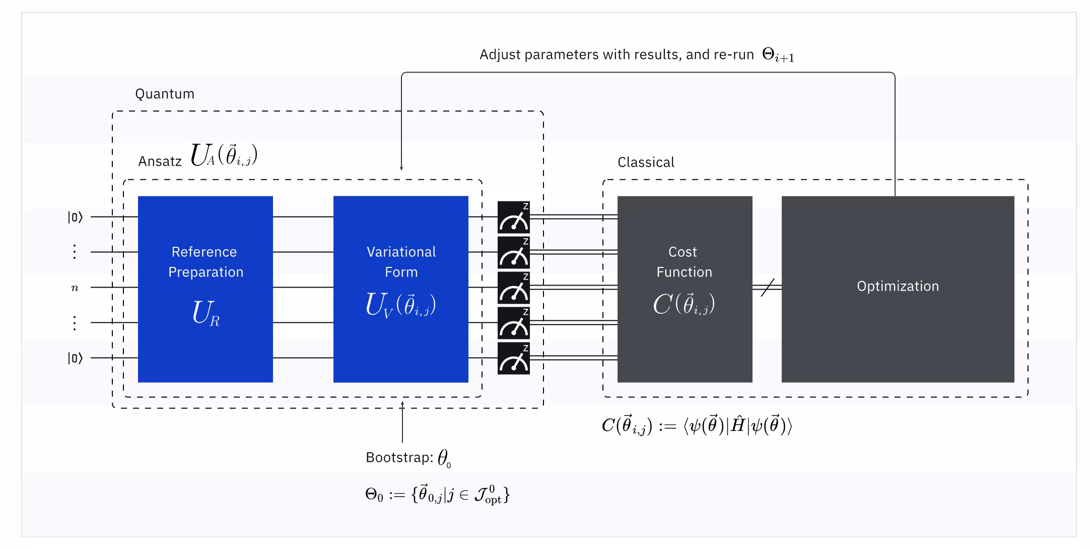
(Quantum) Observable: Ang molecular Hamiltonian (enerhiya ng isang molekula)

Sa VQE, ang molecular/atomic Hamiltonian ay isang observable, ibig sabihin, maaari nating sukatin ang halaga nito sa pamamagitan ng isang eksperimento. Ang aming layunin ay mahanap ang pinakamababang posibleng enerhiya (ang ground state energy) ng molekula. Upang magawa ito, gumagamit tayo ng isang trial quantum state, na nabuo ng isang parameterized quantum circuit (ansatz). Sinusukat natin ang observable at ino-optimize ang quantum state hanggang sa maabot natin ang pinakamababang posibleng enerhiya.

Ang basis set na ginamit para sa molecular Hamiltonian ay nagtatakda ng bilang ng mga qubit na kailangan at direktang nakakaapekto sa katumpakan ng VQE. Ang pagpili ng tamang basis set ay kritikal para sa pagbabalanse ng kahusayan at katumpakan. Upang gawing simple ang mga kalkulasyon nang hindi binabago ang basis set, maaari tayong gumamit ng mga estratehiya tulad ng pagpapatupad ng symmetry at active space reduction. Maraming molekula ang may simetriko na hugis (tulad ng isang mariposa o snowflake), ibig sabihin, ang ilang bahagi ay kumikilos sa parehong paraan. Sa halip na kalkulahin ang lahat nang hiwalay, maaari tayong mag-focus lamang sa mga natatanging bahagi, na nagtitipid ng quantum resources, kaya ginagamit ang symmetry. Sa active space reduction, isinasaalang-alang lamang natin ang mga mahalagang orbital, dahil hindi lahat ng elektron ay makabuluhang nakakaapekto sa molecular energy. Ang mga elektron na malapit sa nucleus ay nananatiling halos hindi nagbabago, habang ang iba ay nakakaimpluwensya sa bonding. Sa pamamagitan ng paglalapat ng mga pamamaraang ito, maaari nating gawing mas mahusay ang VQE habang pinapanatili ang katumpakan.

Kapag nakuha na natin ang molecular Hamiltonian gamit ang wastong basis set at mga estratehiyang nabanggit, kailangan nating i-transform ang Hamiltonian na ito sa isa na angkop para sa mga quantum computer. Ang pag-map ng mga problema sa Pauli operators ay maaaring maging kumplikado. Ito ay lalong totoo sa quantum chemistry, na gumagana sa mga hindi makilalang particle (mga elektron), dahil ang mga qubit ay natatangi. Hindi tayo magdedetalye ng mga mapping dito, ngunit tinutukoy namin kayo sa mga sumusunod na resources. Ang isang pangkalahatang talakayan ng pag-map ng isang problema sa mga quantum operator ay matatagpuan sa Quantum computing in practice. Ang isang mas detalyadong talakayan sa pag-map ng mga problema sa chemistry sa mga quantum operator ay matatagpuan sa Quantum chemistry with VQE.

Para sa modyul na ito, ibibigay namin sa inyo ang angkop na (one-qubit) Hamiltonian para sa $H$ at $H_2$ upang makapag-focus tayo sa paggamit ng quantum computer. Ang mga one-qubit Hamiltonian na ito ay inihanda gamit ang STO-6G basis set at ang Jordan-Wigner mapping, na siyang pinaka-straightforward na mapping na may pinakasimpleng physical interpretation, dahil ini-map nito ang occupancy ng isang spin-orbital sa occupancy ng isang qubit. Gayundin, gumamit tayo ng qubit reduction technique sa pamamagitan ng paggamit ng isang symmetry ng Hamiltonian, na gumagamit ng mga pattern sa kung paano kumikilos ang mga spin occupation upang bawasan ang bilang ng mga qubit. Para sa $H_2$ molecule, ipinapalagay natin na ang distansya sa pagitan ng dalawang hydrogen atom ay 0.735 $\mathring A$.

(Quantum) Ansatz: Ang trial wave function (Paano bumuo ng isang simpleng quantum state gamit ang isang quantum circuit)

Para sa VQE, ang ansatz (maramihan: ansätze) ay binubuo ng dalawang pangunahing bahagi. Ang una ay initial state preparation, na nagse-set up ng state ng qubit sa pamamagitan ng pag-apply ng mga quantum gate nang walang variational parameter. Ang pangalawang bahagi ay ang parameterized quantum circuit, isang espesyal na quantum circuit na may mga adjustable parameter, katulad ng mga dyal sa isang radyo. Ang mga parameter na ito ay gagamitin para sa huling bahagi — ang klasikal na optimizer — upang matulungan tayong maabot ang pinakamahusay na posibleng ground state.

Sa seksyon ng variational principle, natutunan natin na ang kalidad ng trial state ay nakakaapekto sa kalidad ng mga resulta ng variational algorithm. Ibig sabihin, mahalaga ang pagpili ng magandang ansatz sa VQE. Muli, ito ay isang mayaman at kumplikadong paksa. Hindi natin sasaklawin dito ang iba't ibang uri ng ansatz o ang kanilang mga pinagmulan. Kung interesado kang matuto nang higit pa tungkol sa mga parameterized quantum circuit at ansatz, maaari mong tuklasin ang aralin na Ansatz and variational form mula sa Variational algorithm design course, na nagbibigay ng mga detalyadong paliwanag at halimbawa ng mga ansätze.

Dahil gagamit tayo ng one-qubit Hamiltonian sa modyul na ito, kailangan natin ng one-qubit parameterized quantum circuit bilang ansatz. Makikita natin ang tatlong uri ng one-qubit ansätze sa susunod na seksyon. Ikukumpara natin ang mga ito at tatalakayin ang mga pangunahing pagsasaalang-alang sa pagpili ng ansatz.

(Klasikal) Optimizer: pag-fine-tune ng quantum circuit

Kapag nasukat na ng quantum computer ang enerhiya ng observable mula sa ansatz, ang mga parameter ng ansatz at ang halaga ng enerhiya ay ipinapadala sa klasikal na optimizer para sa pag-tune. Ang proseso ng optimization na ito ay isinasagawa sa isang klasikal na computer, karaniwang gumagamit ng mga general-purpose na siyentipikong package tulad ng SciPy.

Tinatrato ng klasikal na optimizer ang nasukat na enerhiya bilang isang cost function. Sa mga problema sa optimization, ang isang cost function (tinatawag ding objective function) ay isang mathematical function na sumusukat kung gaano "kaganda" ang isang partikular na solusyon. Ang layunin ng optimizer ay mahanap ang hanay ng mga parameter na nag-mi-minimize ng cost function na ito. Sa konteksto ng paghahanap ng ground state energy ng isang molekula, ang enerhiya mismo ang nagsisilbing cost function — gusto nating mahanap ang mga parameter para sa ating quantum circuit (ang ating "solusyon") na nagbubunga ng pinakamababang posibleng enerhiya. Ginagamit ng klasikal na optimizer ang nasukat na halagang ito ng enerhiya (ang cost) at tinutukoy ang susunod na hanay ng mga na-optimize na parameter para sa quantum ansatz. Ang mga na-update na parameter na ito ay ibinabalik sa quantum circuit, at ang proseso ay inuulit. Sa bawat iteration, ina-adjust ng klasikal na optimizer ang mga parameter upang subukang bawasan ang enerhiya (i-minimize ang cost function) hanggang sa matugunan ang isang paunang natukoy na convergence criterion, na ideyal na tinitiyak na ang pinakamababang posibleng enerhiya (na tumutugma sa ground state ng molekula para sa bond distance at basis set na iyon) ay natagpuan.

Maraming mga estratehiya ng optimization ang ibinibigay ng mga siyentipikong package tulad ng SciPy. Makakakita ka ng higit pa sa aralin na Optimization loops ng kursong Variational algorithm design. Dito gagamit tayo ng COBYLA (Constrained Optimization BY Linear Approximations), isang optimization algorithm na angkop para sa mga kumplikadong energy landscape. Sa partikular, hindi sinusubukan ng COBYLA na kalkulahin ang gradient ng function na pinag-aaralan; ito ay tinatawag na gradient-free optimizer. Isipin mong sinusubukan mong mahanap ang pinakamataas na tuktok sa isang hanay ng bundok nang nakasara ang iyong mga mata. Dahil hindi mo makita ang buong landscape, gumagawa ka ng maliliit na hakbang sa iba't ibang direksyon, habang sinisuri kung pataas o pababa ka. Gumagana ang COBYLA sa katulad na paraan — gumagalaw ito sa parameter space, sinusubukan ang iba't ibang halaga, unti-unting pinapabuti ang resulta hanggang sa mahanap nito ang pinakamabuti.

Handa ka na ngayon para magsagawa ng VQE calculation. Para doon, subukan ang check-in question sa ibaba, na nagbubuod sa kabuuang proseso.

Suriin ang iyong pag-unawa

Punan ang mga patlang ng tamang termino upang makumpleto ang buod ng proseso ng VQE.

Ang VQE ay isang variational quantum algorithm, na pinagsasama ang kapangyarihan ng (1) ________ at klasikal na computing, na ginagamit upang mahanap ang (2) __________ ng isang molekula. Ang proseso ay nagsisimula sa pamamagitan ng pagtukoy sa (3) __________, na kumakatawan sa kabuuang enerhiya ng sistema at nagsisilbing observable sa mga quantum measurement. Susunod, naghahanda tayo ng isang (4) __________, isang quantum circuit na may mga adjustable parameter na kumakatawan sa trial wave function ng molekula. Ang mga parameter na ito ay ino-optimize gamit ang isang (5) __________, isang klasikal na algorithm na paulit-ulit na nag-a-adjust ng mga parameter upang i-minimize ang nasukat na enerhiya. Sa talakayan sa itaas ginamit namin ang (6) __________ optimizer, na pinipino ang mga parameter ng ansatz nang hindi nangangailangan ng mga derivative calculation. Nagpapatuloy ang proseso hanggang maabot natin ang (7) __________, ibig sabihin, natagpuan na natin ang pinakamababang posibleng enerhiya ng molekula.

Word Bank:

• classical optimizer
• ground state energy
• hardware-efficient
• ansatz
• molecular Hamiltonian
• COBYLA
• quantum computing
• convergence

Sagot:

1 → quantum computing

2 → ground state energy

3 → molecular Hamiltonian

4 → ansatz

5 → classical optimizer

6 → COBYLA

7 → convergence

Kalkulahin ang ground state energy ng isang hydrogen atom gamit ang VQE

Ngayon, gamitin natin ang natutunan natin para kalkulahin ang ground state energy ng isang hydrogen atom. Sa buong modyul, gagamit tayo ng isang balangkas para sa quantum computing na kilala bilang "Qiskit patterns", na hinahati ang mga workflow sa mga sumusunod na hakbang:

• Hakbang 1: I-map ang mga klasikal na input sa isang quantum na problema
• Hakbang 2: I-optimize ang problema para sa quantum na pagpapatupad
• Hakbang 3: Isagawa gamit ang mga Qiskit Runtime primitives
• Hakbang 4: Post-processing at klasikal na pagsusuri

Susundin natin ang mga hakbang na ito sa pangkalahatan.

Magsimula tayo sa pag-load ng ilang kinakailangang mga pakete, kasama na ang mga Qiskit Runtime primitives. Pipili rin tayo ng pinaka-hindi abala na quantum computer na magagamit natin.

May code sa ibaba para sa pag-save ng iyong mga kredensyal sa unang paggamit. Tiyaking burahin ang impormasyong ito mula sa notebook pagkatapos itong i-save sa iyong kapaligiran, para hindi aksidenteng maibahagi ang iyong mga kredensyal kapag ibinabahagi mo ang notebook. Tingnan ang I-set up ang iyong IBM Cloud account at I-initialize ang serbisyo sa isang hindi pinagkakatiwalaang kapaligiran para sa karagdagang gabay.

# Load the Qiskit Runtime service
from qiskit_ibm_runtime import QiskitRuntimeService

# Load the Runtime primitive and session
from qiskit_ibm_runtime import EstimatorV2 as Estimator

# Syntax for first saving your token.  Delete these lines after saving your credentials.
# QiskitRuntimeService.save_account(channel='ibm_quantum_platform', instance = '<YOUR_IBM_INSTANCE_CRN>', token='<YOUR-API_KEY>', overwrite=True, set_as_default=True)
# service = QiskitRuntimeService(channel='ibm_quantum_platform')

# Load saved credentials
service = QiskitRuntimeService()

# Use the least busy backend, or uncomment the loading of a specific backend like "ibm_brisbane".
backend = service.least_busy(operational=True, simulator=False, min_num_qubits=127)
# backend = service.backend("ibm_brisbane")
print(backend.name)

ibm_brisbane

Ang cell sa ibaba ay magbibigay-daan sa iyo na lumipat sa pagitan ng paggamit ng simulator o totoong hardware sa buong notebook. Inirerekumenda naming patakbuhin ito ngayon:

# Load the Aer simulator and generate a noise model based on the currently-selected backend.
from qiskit_aer import AerSimulator
from qiskit_aer.noise import NoiseModel

# Alternatively, load a fake backend with generic properties and define a simulator.

noise_model = NoiseModel.from_backend(backend)

# Define a simulator using Aer, and use it in Sampler.
backend_sim = AerSimulator(noise_model=noise_model)

Hakbang 1: I-map ang problema sa mga quantum circuit at operator

Sisimulan natin ang ating VQE na kalkulasyon sa pamamagitan ng pagtatakda ng Hamiltonian para sa hydrogen molecule ($H_2$) sa isang tiyak na distansya ng bond. Kinakatawan ng Hamiltonian na ito ang kabuuang enerhiya ng sistema sa mga tuntunin ng qubit operator, na nagmula at na-map mula sa molecular na sistema gamit ang isang karaniwang pamamaraan: 1) paggamit ng STO-6G basis set (isang tiyak na koleksyon ng mga mathematical na function na ginagamit upang aproksimasyunin ang mga electron orbital), 2) paglalapat ng Jordan-Wigner mapping (isang teknik para isalin ang mga fermionic operator na naglalarawan ng mga elektron sa mga qubit operator), at 3) pagsasagawa ng qubit reduction gamit ang mga simetriya ng Hamiltonian upang pasimplehin ang problema.

Tulad ng ipinaliwanag natin kanina, ang mga kinakalkula na ground state energy ay lubos na nakasalalay sa pagpili ng basis set at sa molecular geometry (tulad ng distansya ng bond). Para sa partikular na configuration na ito at pagkatapos ng mga transformation na ito, ang nagresultang qubit Hamiltonian ay simple:

$\hat{H} = -0.2355 I + 0.2355 Z$

Dito, ang $I$ ay kumakatawan sa identity operator at ang $Z$ ay kumakatawan sa Pauli-Z operator, na kumikilos sa isang solong qubit. Ang mga coefficient ay nagmula sa mga integral na kinalkula gamit ang STO-6G basis set sa partikular na distansya ng bond na ito na may wastong transformation.

Kapag natukoy na ang Hamiltonian na ito, maaari na nating gamitin ang VQE para kalkulahin ang ground state energy nito. Kapaki-pakinabang na ihambing ang ating kinakalkula na ground state energy sa mga inaasahang halaga. Para sa isang solong, nag-iisang hydrogen atom (H), ang ground state energy ay eksaktong -0.5 Hartree (sa kawalan ng mga relativistic na epekto). Kalkulahin natin ang eksaktong ground state energy ng ating tiyak na qubit Hamiltonian gaya ng tinukoy sa itaas at ihambing ito sa mga kaugnay na kilalang halaga.

from qiskit.quantum_info import SparsePauliOp
import numpy as np

# Qubit Hamiltonian of the hydrogen atom generated by using STO-3G basis set and parity mapping
Hamiltonian = SparsePauliOp.from_list([("I", -0.2355), ("Z", 0.2355)])

# exact ground state energy of Hamiltonian

A = np.array(Hamiltonian)
eigenvalues, eigenvectors = np.linalg.eig(A)
print(
    "The exact ground state energy of the Hamiltonian is ",
    min(eigenvalues).real,
    "hartree",
)
h = min(eigenvalues.real)

The exact ground state energy of the Hamiltonian is  -0.471 hartree

Susunod, kailangan natin ng isang parameterized quantum circuit, isang ansatz, para maghanda ng trial wave function na $\Psi_\text{trial}$ para sa ground state. Ang layunin ay hanapin ang mga parameter na $\theta$ na nagpapababa ng energy expectation value na $\langle\psi(\theta)|\hat{H}|\psi(\theta)\rangle$. Ang pagpili ng ansatz ay napakahalaga dahil tinutukoy nito ang hanay ng mga posibleng quantum state na maaaring ihanda ng ating circuit. Ang isang "magandang" ansatz ay sapat na nababaluktot para kumatawan sa isang estado na malapit na malapit sa tunay na ground state ng Hamiltonian na ating pinag-aaralan, ngunit hindi masyadong kumplikado na nangangailangan ng masyadong maraming parameter o masyadong malalim na circuit para sa mga kasalukuyang quantum computer.

Dito, susubukan natin ang tatlong magkakaibang one-qubit na ansätze para makita kung alin ang nagbibigay ng mas magandang "saklaw" ng mga posibleng quantum state na maaaring nasa isang solong qubit. Ang "saklaw" ay tumutukoy sa hanay ng mga quantum state na maaaring malikha ng ansatz circuit sa pamamagitan ng pagbabago ng mga parameter nito.

Gagamit tayo ng tatlong ansätze batay sa iba't ibang kombinasyon ng mga single-qubit rotational gate:

• Isang 1-axis rotational gate ansatz: Gumagamit ang ansatz na ito ng mga pag-ikot sa paligid ng isang axis lamang ($R_x(\theta)$). Sa Bloch sphere, tumutugma ito sa paggalaw sa isang tiyak na bilog lamang. Ito ang pinaka-hindi nababaluktot at sumasaklaw sa limitadong hanay ng mga estado.
• Dalawang 2-axis rotational gate ansätze: Pinagsasama ng mga ansätze na ito ang mga pag-ikot sa paligid ng dalawang magkaibang axis ($R_x(\theta_1) R_z(\theta_2)$ at $R_x(\theta_1) R_z(\theta_2) R_x(\theta_3)$). Nagbibigay-daan ito sa atin na maabot ang mas malaking bahagi ng Bloch sphere, kumpara sa isang single-axis rotation.

Sa pamamagitan ng paghahambing ng mga resulta ng VQE na nakuha gamit ang tatlong ansätze na ito, makikita natin kung paano nakakaapekto ang flexibility at state-space coverage ng ansatz sa ating kakayahang mahanap ang tunay na ground state energy ng ating pinasimpleng Hamiltonian. Ang mas nababaluktot na ansatz ay may potensyal na makahanap ng mas magandang aproksimyon, ngunit maaari rin itong maging mas mahirap para sa klasikal na optimizer.

from qiskit import QuantumCircuit
from qiskit.circuit import Parameter
from qiskit.quantum_info import Statevector, DensityMatrix, Pauli

theta = Parameter("θ")
phi = Parameter("φ")
lam = Parameter("λ")

ansatz1 = QuantumCircuit(1)
ansatz1.rx(theta, 0)

ansatz2 = QuantumCircuit(1)
ansatz2.rx(theta, 0)
ansatz2.rz(phi, 0)

ansatz3 = QuantumCircuit(1)
ansatz3.rx(theta, 0)
ansatz3.rz(phi, 0)
ansatz3.rx(lam, 0)

<qiskit.circuit.instructionset.InstructionSet at 0x1059def80>

Ngayon, bumuo tayo ng 5000 random na numero para sa bawat parameter at i-plot ang distribusyon ng mga random na quantum state, na nabuo ng tatlong ansätze gamit ang mga random na parameter na ito. Maaari mong isipin ang mga parameter na ito bilang mga pag-ikot sa paligid ng iba't ibang axis sa isang spherical na ibabaw. Para makita ang distribusyon ng quantum state, gagamit tayo ng the Bloch Sphere, isang three-dimensional na bola na nagpapakita ng estado ng isang solong qubit. Ang anumang punto sa bola ay kumakatawan sa isang posibleng estado ng qubit, kung saan ang hilaga at timog na polo ay parang klasikal na "0" at "1", ngunit ang qubit ay maaari rin nasa kahit saan sa pagitan, na nagpapakita ng mga espesyal na quantum na katangian tulad ng superposition. Una, ihanda ang mga kinakailangang function para i-plot ang 3D Bloch sphere at maghanda ng 5000 random na parameter.

import matplotlib.pyplot as plt

def plot_bloch(bloch_vectors):
    # Extract X, Y, Z coordinates for 3D projection
    X_coords = bloch_vectors[:, 0]
    Z_coords = bloch_vectors[:, 2]

    # Compute Y coordinates from X and Z to approximate the full Bloch sphere projection
    Y_coords = bloch_vectors[:, 1]

    # Create 3D plot
    fig = plt.figure(figsize=(8, 8))
    ax = fig.add_subplot(111, projection="3d")
    ax.scatter(X_coords, Y_coords, Z_coords, color="blue", alpha=0.6)

    # Labels and title
    ax.set_xlabel("X")
    ax.set_ylabel("Y")
    ax.set_zlabel("Z")
    ax.set_title("Parameterized 1-Qubit Circuit on 3D Bloch Sphere")

    # Set axis limits and make them equal
    ax.set_xlim([-1, 1])
    ax.set_ylim([-1, 1])
    ax.set_zlim([-1, 1])

    # Ensure equal aspect ratio for all axes
    ax.set_box_aspect([1, 1, 1])  # Equal scaling for x, y, z axes

    # Show grid
    ax.grid(True)

    plt.show()

num_samples = 5000  # Number of random states
theta_vals = np.random.uniform(0, 2 * np.pi, num_samples)
phi_vals = np.random.uniform(0, 2 * np.pi, num_samples)
lam_vals = np.random.uniform(0, 2 * np.pi, num_samples)

Tingnan natin kung paano gumagana ang ating unang ansatz.

# List to store Bloch Sphere XZ coordinates
bloch_vectors = []

# Generate quantum states and extract Bloch vectors
for i in range(num_samples):
    # Create a circuit and bind parameters
    qc = ansatz1
    bound_qc = qc.assign_parameters({theta: theta_vals[i]})  # , lam: lam_vals[i]})
    state = Statevector.from_instruction(bound_qc)
    rho = DensityMatrix(state)

    X = rho.expectation_value(Pauli("X")).real
    Y = rho.expectation_value(Pauli("Y")).real
    Z = rho.expectation_value(Pauli("Z")).real
    bloch_vectors.append([X, Y, Z])  # Store X, Z components

# Convert to a numpy array for plotting
bloch_vectors = np.array(bloch_vectors)

plot_bloch(bloch_vectors)

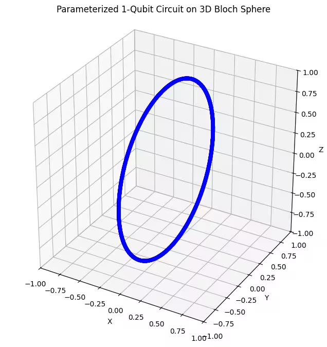
Makikita natin na ang ating unang ansatz ay nagbabalik ng ring-shaped na distribusyon ng mga quantum state sa Bloch sphere. May katuturan ito, dahil isa lamang na rotational na parameter ang ibinigay natin sa ansatz. Kaya naman, makakagawa lamang ito ng mga estado na inikot sa paligid ng isang axis. Ang pagsisimula mula sa punto na $(0,0,1)$ at pag-ikot sa paligid ng isang axis ay palaging magbubunga ng isang singsing. Saka naman, tingnan natin ang ating ikalawang ansatz, na may dalawang orthogonal na rotational gate — Rx at Rz.

bloch_vectors = []

# Generate quantum states and extract Bloch vectors
for i in range(num_samples):
    # Create circuit and bind parameters
    qc = ansatz2
    bound_qc = qc.assign_parameters(
        {theta: theta_vals[i], phi: phi_vals[i]}
    )  # , lam: lam_vals[i]})
    state = Statevector.from_instruction(bound_qc)
    rho = DensityMatrix(state)

    X = rho.expectation_value(Pauli("X")).real
    Y = rho.expectation_value(Pauli("Y")).real
    Z = rho.expectation_value(Pauli("Z")).real
    bloch_vectors.append([X, Y, Z])  # Store X, Z components

# Convert to numpy array for plotting
bloch_vectors = np.array(bloch_vectors)

plot_bloch(bloch_vectors)

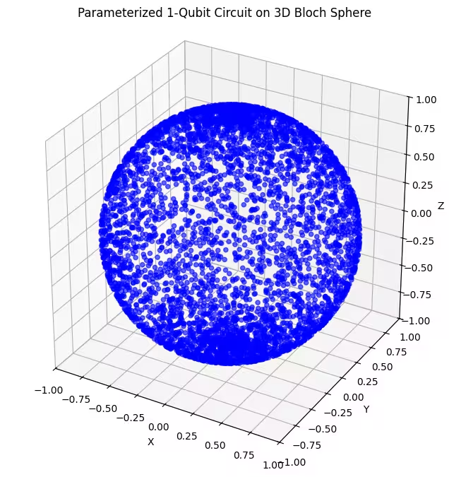
Dito, makikita natin na ang ating ikalawang ansatz ay sumasaklaw ng mas malaking bahagi ng Bloch sphere — ngunit pansinin na mas nakakonsentrate ang mga tuldok sa paligid ng mga polo at mas kalat sa paligid ng ekwador. Oras na para suriin ang ating huling ansatz.

bloch_vectors = []

# Generate quantum states and extract Bloch vectors
for i in range(num_samples):
    # Create circuit and bind parameters
    qc = ansatz3
    bound_qc = qc.assign_parameters(
        {theta: theta_vals[i], phi: phi_vals[i], lam: lam_vals[i]}
    )
    state = Statevector.from_instruction(bound_qc)
    rho = DensityMatrix(state)

    X = rho.expectation_value(Pauli("X")).real
    Y = rho.expectation_value(Pauli("Y")).real
    Z = rho.expectation_value(Pauli("Z")).real
    bloch_vectors.append([X, Y, Z])  # Store X, Z components

# Convert to numpy array for plotting
bloch_vectors = np.array(bloch_vectors)

plot_bloch(bloch_vectors)

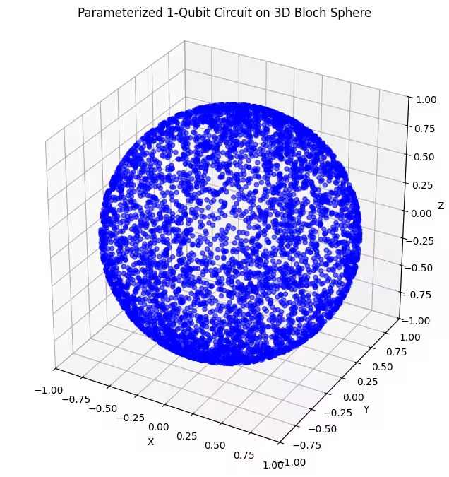
Dito makikita mo ang mas pantay na distribusyon ng mga quantum state na nabuo ng ating huling ansatz.

Tulad ng nabanggit, ang pinakamabuting gawin ay ang makakuha ng kaalaman tungkol sa ground state na iyong hinahanap at gumamit ng ansatz na angkop para suriin ang mga estado na malapit sa ground state na iyon. Halimbawa, kung alam natin na ang ating ground state ay malapit sa isang polo, maaaring piliin natin ang ansatz 2. Para sa kasimplihan, mananatili tayo sa ansatz 3, na pantay na sinisiyasat ang buong Bloch sphere.

Ngayon na napili na natin ang ating ansatz, i-draw natin ang circuit.

# Pre-defined ansatz circuit and operator class for Hamiltonian

ansatz = ansatz3

num_params = ansatz.num_parameters
print("This circuit has ", num_params, "parameters")

ansatz.draw("mpl", style="iqp")

This circuit has  3 parameters

Hakbang 2: I-optimize para sa target na hardware

Kapag nagpapatakbo ng kalkulasyon sa isang totoong quantum computer, hindi lang natin iniisip ang lohika ng quantum circuit. Isinasaalang-alang din natin ang mga bagay tulad ng kung anong mga operasyon ang maaaring isagawa ng partikular na quantum computer na iyon, at kung saan sa quantum computer naroon ang mga qubit na ginagamit natin. Magkatabing-katabi ba sila? Malayo ba sa isa't isa? Kaya naman, ang susunod na hakbang ay ang muling isulat ang ating circuit gamit ang mga gate na natural para sa quantum computer na gagamitin natin, at isinasaalang-alang ang layout ng qubit. Magagawa ito sa pamamagitan ng transpilation — pagkatapos ng prosesong ito, makikita mo ang ating simpleng ansatz na na-convert sa ibang hanay ng mga gate, at ang ating mga abstract na qubit ay maimamapa sa mga pisikal na qubit sa isang totoong quantum computer.

from qiskit.transpiler.preset_passmanagers import generate_preset_pass_manager

config = backend.configuration()

print("Backend: {config.backend_name}")
print("Native gates: ", config.supported_instructions, ",")

target = backend.target

pm = generate_preset_pass_manager(target=target, optimization_level=3)

ansatz_isa = pm.run(ansatz)

ansatz_isa.draw(output="mpl", idle_wires=False, style="iqp")

Backend: {config.backend_name}
Native gates:  ['ecr', 'id', 'delay', 'measure', 'reset', 'rz', 'sx', 'x'] ,

Makikita mo na ang mga rx, rz gate ng ating ansatz ay na-convert sa isang serye ng rz, sx gate, na siyang mga native gate ng ating backend. Makikita mo rin na ang ating q0 ay naimapa na ngayon sa ikalimang pisikal na qubit. Kailangan din nating i-map ang ating Hamiltonian ayon sa mga pagbabagong ito, tulad ng sa sumusunod na code:

Hamiltonian_isa = Hamiltonian.apply_layout(layout=ansatz_isa.layout)

Hakbang 3: Isagawa sa target na hardware

Oras na para patakbuhin ang ating VQE sa isang totoong QPU. Para dito, kailangan muna natin ng cost function para sa proseso ng optimization, na sinusuri ang expectation value ng Hamiltonian gamit ang isang quantum state na nabuo ng ansatz. Huwag mag-alala! Hindi mo kailangang i-code ang lahat nang mag-isa. Naghanda kami ng function para dito, at ang kailangan mo lang gawin ay patakbuhin ang cell sa ibaba.

def cost_func(params, ansatz, hamiltonian, estimator):
    """Return estimate of energy from estimator

    Parameters:
        params (ndarray): Array of ansatz parameters
        ansatz (QuantumCircuit): Parameterized ansatz circuit
        hamiltonian (SparsePauliOp): Operator representation of Hamiltonian
        estimator (EstimatorV2): Estimator primitive instance
        cost_history_dict: Dictionary for storing intermediate results

    Returns:
        float: Energy estimate
    """
    pub = (ansatz, [hamiltonian], [params])
    result = estimator.run(pubs=[pub]).result()
    energy = result[0].data.evs[0]

    cost_history_dict["iters"] += 1
    cost_history_dict["prev_vector"] = params
    cost_history_dict["cost_history"].append(energy)
    print(f"Iters. done: {cost_history_dict['iters']} [Current cost: {energy}]")

    return energy

Sa wakas, ihahanda natin ang mga paunang parameter para sa ating ansatz at sa proseso ng optimization nito. Maaari kang simpleng gumamit ng lahat ng zero o random na halaga. Pinili namin ang mga paunang parameter sa ibaba, ngunit huwag mag-atubiling mag-comment o mag-uncomment ng mga linya sa cell para random na mag-sample ng mga parameter, pantay mula 0 hanggang $2\pi$.

# x0 = np.random.uniform(0, 2*pi, 3)
x0 = [1, 1, 0]

# QPU Est. 2min for ibm_brisbane

from scipy.optimize import minimize
from qiskit_ibm_runtime import Batch

batch = Batch(backend=backend)

cost_history_dict = {
    "prev_vector": None,
    "iters": 0,
    "cost_history": [],
}
estimator = Estimator(mode=batch)
estimator.options.default_shots = 10000

res = minimize(
    cost_func,
    x0,
    args=(ansatz_isa, Hamiltonian_isa, estimator),
    method="cobyla",
    options={"maxiter": 10, "tol": 0.01},
)

batch.close()

Iters. done: 1 [Current cost: -0.3361517318448143]
Iters. done: 2 [Current cost: -0.4682546422099432]
Iters. done: 3 [Current cost: -0.38985802144149584]
Iters. done: 4 [Current cost: -0.38319217316749354]
Iters. done: 5 [Current cost: -0.4628720756579032]
Iters. done: 6 [Current cost: -0.4683301936226905]
Iters. done: 7 [Current cost: -0.45480498699294747]
Iters. done: 8 [Current cost: -0.4690533242050814]
Iters. done: 9 [Current cost: -0.465867415110354]
Iters. done: 10 [Current cost: -0.4606882723137227]

h_vqe = res.fun
print("The reference ground state energy is ", min(eigenvalues))
print("The computed ground state energy is ", h_vqe)

The reference ground state energy is  (-0.471+0j)
The computed ground state energy is  -0.4690533242050814

Binabati kita! Matagumpay mo na ngayong natapos ang iyong unang quantum chemistry na eksperimento. Makikita natin ang pagkakaiba sa pagitan ng eksaktong ground state energy ng Hamiltonian at sa atin, ngunit dahil gumamit tayo ng default na error mitigation technique (na nagwawasto ng mga readout error), maliit lamang ang pagkakaiba. Napakagandang simula nito!

Tandaan: Maaari kang makakuha ng mas magandang resulta sa pamamagitan ng pagtatakda ng antas ng error mitigation gamit ang resilience_level. Ang default na halaga ay 1, at kung magtakda ka ng mas mataas na halaga, gagamit ito ng mas maraming oras ng QPU ngunit maaaring magbalik ng mas magandang resulta.

Hakbang 4: Post-process

Oras na para tingnan kung paano gumana ang ating klasikal na optimizer. Patakbuhin ang cell sa ibaba at tingnan ang pattern ng convergence.

fig, ax = plt.subplots()
x = np.linspace(0, 10, 10)

# Define the constant function
y_constant = np.full_like(x, h)
ax.plot(
    range(cost_history_dict["iters"]), cost_history_dict["cost_history"], label="VQE"
)
ax.set_xlabel("Iterations")
ax.set_ylabel("Cost (Hartree)")
ax.plot(y_constant, label="Target")
plt.legend()
plt.draw()

Nagsimula tayo sa isang medyo magandang paunang halaga, kaya nakakuha tayo ng magandang panghuling halaga sa loob lamang ng 10 hakbang. Makikita mo ang malalaki at maliliit na tuktok, at ito ang tipikal na katangian ng COBYLA optimizer — hinahanap nito ang espasyo na parang hindi nito makita ang landscape at inaayos ang mga laki ng hakbang sa bawat pagsukat.

Suriin ang iyong pag-unawa

Ano ang iyong obserbasyon? Alin sa mga bahagi ng proseso sa itaas ang bukas sa pagpapabuti upang makakuha ng mga resulta na mas malapit sa mga teoretikal na halaga, o mas malapit sa tumpak na ground state energy ng Hamiltonian? Ano ang ilang bagay na dapat isaalang-alang para dito?

Sagot:

Ang unang dapat isaalang-alang ay ang pagbabago sa hanay ng mga base na ginagamit sa pagkalkula ng Hamiltonian ng mga molekula. Tulad ng nabanggit kanina, ang ground state energy ng H atom ay -0.5 Hartree, gaya ng kilala, at ang STO-6G basis na pinili natin ay hindi sapat para tumpak na makuha ang halagang ito.

Ang pagpili ng mas kumplikadong uri ng basis ay nagdadagdag ng bilang ng mga qubit na ginagamit ng Hamiltonian; kaya naman, kailangan nating pumili ng mas kumplikado at angkop na ansatz para sa mga problema sa chemistry.

Ang susunod na dapat i-optimize ay ang pamamahala ng ingay sa QPU. Ang mas advanced na mga teknik ng error mitigation ay nagbubunga ng mas magandang resulta ngunit maaaring mas matagal gamitin. Isaalang-alang din kung paano nakakaapekto ang shot_number sa mga resulta.

Sa wakas, mas magandang convergence performance ay maaari ring makamit sa pamamagitan ng pagsubok ng iba't ibang optimizer.

Kalkulahin ang ground state energy ng hydrogen molecule gamit ang VQE

Ngayon na napag-aralan na natin ang pangkalahatang proseso ng VQE gamit ang mga $H$ atom, kakalkulahin na natin ang ground state energy ng molekulang $H_2$ nang mas mabilis.

Hakbang 1: I-map ang problema sa quantum circuits at operators

Ibinibigay din namin dito ang isang one-qubit Hamiltonian na gumagamit ng STO-6G basis at ng Jordan-Wigner transformation, na may qubit reduction sa pamamagitan ng isang symmetry ng Hamiltonian. Tandaan na ginamit namin ang atomic distance na 0.735 $\mathring A$ sa pagitan ng dalawang hydrogen atom.

Hindi tulad ng pagkalkula para sa isang hydrogen atom ($H$), para makuha ang ground state ng hydrogen molecule ($H_2$), kailangan din naming isaalang-alang ang repulsive force sa pagitan ng mga nucleus ng dalawang hydrogen atom, bukod sa energy na nauugnay sa mga electronic orbital. Sa hakbang na ito, ibibigay natin ang halagang ito bilang constant, at talagang kakalkulahin natin ang halagang ito sa check-in problem.

$\hat{H} = -1.04886 I + -0.79674 Z + 0.18122 X$

h2_hamiltonian = SparsePauliOp.from_list(
    [("I", -1.04886087), ("Z", -0.7967368), ("X", 0.18121804)]
)

# exact ground state energy of hamiltonian
nuclear_repulsion = 0.71997
A = np.array(h2_hamiltonian)
eigenvalues, eigenvectors = np.linalg.eig(A)
print("Electronic ground state energy (Hartree): ", min(eigenvalues).real)
print("Nuclear repulsion energy (Hartree): ", nuclear_repulsion)
print(
    "Total ground state energy (Hartree): ", min(eigenvalues).real + nuclear_repulsion
)
h2 = min(eigenvalues).real + nuclear_repulsion

Electronic ground state energy (Hartree):  -1.8659468547627318
Nuclear repulsion energy (Hartree):  0.71997
Total ground state energy (Hartree):  -1.1459768547627318

Hakbang 2: I-optimize para sa target na hardware

Dahil pareho ang bilang ng mga qubit na ginagamit ng nakaraang VQE at Hamiltonian at ng backend na gagamitin para sa execution, gagamitin na lang natin ang kasalukuyang ansatz at ang na-optimize na anyo nito.

h2_hamiltonian_isa = h2_hamiltonian.apply_layout(layout=ansatz_isa.layout)

Hakbang 3: I-execute sa target na hardware

Oras na para gawin ang mga kalkulasyon sa aktwal na QPU. Halos pareho ang lahat, ngunit gagamit tayo ng angkop na initial point para tumugma sa Hamiltonian. Gayundin, sa iterative na bahagi, ilang setting ng Estimator — na ginagamit para kalkulahin ang mga expectation ng Hamiltonian para sa ansatz sa QPU — ay bahagyang naiiba mula sa mga nakaraang kalkulasyon. Tatalakayin pa natin ang pagbabagong ito sa check-in question.

x0 = [2, 0, 0]

# QPU time 4min for ibm_brisbane
batch = Batch(backend=backend)

cost_history_dict = {
    "prev_vector": None,
    "iters": 0,
    "cost_history": [],
}
estimator = Estimator(mode=batch)
estimator.options.default_shots = 10000

res = minimize(
    cost_func,
    x0,
    args=(ansatz_isa, h2_hamiltonian_isa, estimator),
    method="cobyla",
    options={"maxiter": 15},
)

batch.close()

Iters. done: 1 [Current cost: -0.710621837568328]
Iters. done: 2 [Current cost: -0.2603208441168329]
Iters. done: 3 [Current cost: -0.25548711201326424]
Iters. done: 4 [Current cost: -0.581129450619904]
Iters. done: 5 [Current cost: -1.722920997605439]
Iters. done: 6 [Current cost: -1.6633324849371915]
Iters. done: 7 [Current cost: -1.8066989598929164]
Iters. done: 8 [Current cost: -1.8051093803839542]
Iters. done: 9 [Current cost: -1.802692217571555]
Iters. done: 10 [Current cost: -1.8233585485263144]
Iters. done: 11 [Current cost: -1.6904116652617205]
Iters. done: 12 [Current cost: -1.8245120321245392]
Iters. done: 13 [Current cost: -1.6837021361383608]
Iters. done: 14 [Current cost: -1.8166632606115467]
Iters. done: 15 [Current cost: -1.863446212658907]

h2_vqe = res.fun + nuclear_repulsion
print(
    "The reference ground state energy is ", min(eigenvalues).real + nuclear_repulsion
)
print("The computed ground state energy is ", h2_vqe)

The reference ground state energy is  -1.1459768547627318
The computed ground state energy is  -1.143476212658907

Sa teorya, ang VQE ay nagbibigay ng upper bound sa tunay na ground state energy. Ngunit sa praktikal na implementasyon sa tunay o maingay na simulated quantum hardware — pati na rin ang mga approximation na ginawa sa paghahanda ng Hamiltonian (tulad ng basis sets o qubit reduction) — maaaring magdulot ng mga error na minsan ay nagreresulta sa sinukat na energy na bahagyang mas mababa kaysa sa eksaktong teoretikal na halaga o sa isang partikular na numerical reference. Kahit may ilang error, ang mga resulta ay mukhang kasiya-siya, lalo na kung isasaalang-alang ang maliit na bilang ng mga hakbang. Ngayon, tapusin na natin ang VQE calculation na ito sa pamamagitan ng pagtingin kung paano gumana ang optimizer.

Hakbang 4: Post-process

fig, ax = plt.subplots()
x = np.linspace(0, 5, 15)

# Define the constant function
y_constant = np.full_like(x, min(eigenvalues))
ax.plot(
    range(cost_history_dict["iters"]), cost_history_dict["cost_history"], label="VQE"
)
ax.set_xlabel("Iterations")
ax.set_ylabel("Cost (Hartree)")
ax.plot(y_constant, label="Target")
plt.legend()
plt.draw()

Suriin ang iyong pag-unawa

Kalkulahin natin ang nuclear repulsion energy ng molekulang $H_2$, na isinama natin bilang constant na halaga (0.71997 Hartree).

Gamitin ang batas ni Coulomb at ang atomic unit para matiyak na makukuha mo ang halaga sa Hartree.

Sagot:

Dahil positibo ang charge ng parehong hydrogen nucleus, nagtutulak sila sa isa't isa dahil sa electrostatic force. Inilalarawan ng batas ni Coulomb ang repulsyon na ito:

$E_{repulsive} = \frac{e^2}{4\pi\epsilon_0R}$,

kung saan ang $e$ ay ang charge ng proton, ang $\epsilon_0$ ay ang vacuum permittivity, at ang $R$ ay ang distansya sa pagitan ng dalawang nucleus, na sinusukat sa metro o Bohr radii sa yunit na joules (J).

Para kalkulahin ang energy na ito sa Hartree, kailangan nating i-convert ang equation sa itaas sa Atomic Unit (AU) system. Sa AU, ang $e^2 = 1$, $4\pi\epsilon_0=1$, at ang Bohr radius ($a_0$) ay 1, at nagiging pangunahing length scale sa AU. Sa mga simplipikasyong ito, nababawasan ang batas ni Coulomb sa:

$E_{repulsion} = \frac{1}{R}$,

kung saan ang $R$ ay dapat na nasusukat sa Bohr radii ($a_0$).

Para i-convert ang ibinigay na nuclear separation sa $\r{A}$ patungong $a_0$, kailangan natin ang conversion relation na ito:

$1\r{A} = 1.88973 a_0$

kaya ang $0.735\r{A}$ ay nagiging $0.735 * 1.88973 = 1.38895 a_0$.

Samakatuwid, ang nuclear repulsion energy ng ibinigay na $H_2$ ay:

$E_{repulsion} = \frac{1}{R} = \frac{1}{1.38895} = 0.71997 Hartree$

Kalkulahin ang reaction energy ng $H + H = H_2$

Gamitin na natin ang ating mga nakuha! Ginamit mo ang VQE, isang variational quantum eigensolver, para kalkulahin ang ground state energy ng $H$ atom at ng molekulang $H_2$. Ang natitira ay gamitin ang mga nakalkulang halaga para makuha ang reaction energy ng prosesong $H + H = H_2$.

Ang reaction energy ay ang pagbabago ng energy na nangyayari kapag ang mga sangkap ay nagre-react para bumuo ng mga bagong sangkap. Isipin mo na nagtatayo ka ng isang bagay: minsan kailangan mong mag-lagay ng energy (tulad ng pag-stack ng mga bloke), at minsan naman ay may napapalabas na energy (tulad ng bola na gumugulong pababa ng burol). Sa kimika, ang mga reaksyon ay alinman sa umaabsorb ng energy (endothermic) o naglalabas ng energy (exothermic).

Ang reaction energy ng prosesong $H + H = H_2$ ay makukuha sa pamamagitan ng sumusunod na formula:

$E_{reaction} = E_{H_2} - (E_H + E_H)$

Sa pamamagitan ng pagpapatakbo ng cell sa ibaba, tingnan natin ito nang biswal. Gagamitin natin dito ang eksaktong ground state value ng bawat Hamiltonian, at ikukumpara natin ang reaction energy ng eksaktong solusyon at ng mga resulta ng VQE.

# Theoretical values
E_H_theo = h.real
E_H2_theo = h2

# Experimental values
E_H_exp = h_vqe
E_H2_exp = h2_vqe

# Calculate reaction energies
E_reaction_theo = E_H2_theo - (2 * E_H_theo)
E_reaction_exp = E_H2_exp - (2 * E_H_exp)

# Set up the plot
fig, ax = plt.subplots(figsize=(8, 6))
ax.set_xlim(0, 3)
ax.set_ylim(-1.16, -0.93)  # Adjust y-axis range to highlight differences
ax.set_xticks([])
ax.set_ylabel("Energy (Hartree)")
ax.set_title("H + H → H₂ Reaction Energy Diagram")

# Plot theoretical energy levels
ax.hlines(
    y=2 * E_H_theo, xmin=0.5, xmax=1.3, linewidth=2, color="r", label="2H (Exact)"
)
ax.hlines(y=E_H2_theo, xmin=1.3, xmax=2, linewidth=2, color="b", label="H₂ (Exact)")

# Plot experimental energy levels
ax.hlines(
    y=2 * E_H_exp,
    xmin=0.5,
    xmax=1.5,
    linewidth=2,
    color="r",
    linestyle="dashed",
    label="2H (VQE)",
)
ax.hlines(
    y=E_H2_exp,
    xmin=1.5,
    xmax=2.5,
    linewidth=2,
    color="b",
    linestyle="dashed",
    label="H₂ (VQE)",
)

# Add labels
ax.text(
    1,
    2 * E_H_theo,
    f"2H: {2*E_H_theo:.4f}",
    verticalalignment="top",
    horizontalalignment="left",
)
ax.text(
    2,
    E_H2_theo,
    f"H₂: {E_H2_theo:.4f}",
    verticalalignment="top",
    horizontalalignment="left",
)
ax.text(
    1,
    2 * E_H_exp,
    f"2H_VQE: {2*E_H_exp:.4f}",
    verticalalignment="bottom",
    horizontalalignment="right",
)
ax.text(
    2,
    E_H2_exp,
    f"H₂_VQE: {E_H2_exp:.4f}",
    verticalalignment="bottom",
    horizontalalignment="right",
)

# Add arrows for reaction energy with ΔE label in the middle
mid_y_theo = (2 * E_H_theo + E_H2_theo) / 2
mid_y_exp = (2 * E_H_exp + E_H2_exp) / 2
ax.annotate(
    "",
    xy=(1.3, E_H2_theo),
    xytext=(1.3, 2 * E_H_theo),
    arrowprops=dict(arrowstyle="<->", color="g"),
)
ax.text(
    1.35, mid_y_theo, f"ΔE: {E_reaction_theo:.4f}", color="g", verticalalignment="top"
)

ax.annotate(
    "",
    xy=(1.5, E_H2_exp),
    xytext=(1.5, 2 * E_H_exp),
    arrowprops=dict(arrowstyle="<->", color="g", linestyle="dashed"),
)
ax.text(
    1.55,
    mid_y_exp,
    f"ΔE_VQE: {E_reaction_exp:.4f}",
    color="g",
    verticalalignment="center",
)

# Add legend
ax.legend()

plt.show()

Gaya ng nakikita sa pigura, kahit may ilang error, ang eksaktong ground state energy ng mga Hamiltonian at ang reaction energy na kinakalkula gamit ang mga resulta ng VQE ay magkakatulad, malapit sa -0.2 Hartree.

Dapat pansinin dito na ang reaction energy ng prosesong ito ay may negatibong halaga, na nangangahulugang ang energy ay napapalabas sa proseso, at ang nabubuo na molekula ay may mas mababang energy kaysa sa dalawang hiwalay na atom.

6. Konklusyon

Buuin natin ang lahat ng ating natutunan.

Una, tiningnan natin ang dalawang mahalagang approximation technique na kailangan para malutas ang mga problema sa quantum chemistry: ang variational principle at ang pagpili ng basis set, na parehong pangunahin sa VQE. Sinuri natin ang variational principle nang pabahay, na kinakalkula ang ground state energy ng simpleng harmonic oscillator.

Susunod, sinuri natin ang VQE, isang malawakang ginagamit na algorithm para kalkulahin ang ground state energy ng isang quantum system. Nagpatakbo tayo ng code para kalkulahin ang mga ground state energy ng atomic hydrogen ($H$) at ng hydrogen molecule ($H_2$). Sa partikular, natutunan natin na kailangan munang makuha ang angkop na molecular Hamiltonian para sa system at i-transform ito sa isang anyo na maaaring i-execute sa isang quantum computer. Nakita rin natin na ang ansatz — isang parameterized quantum circuit — ay kailangan para maghanda ng mga trial quantum state sa loob ng VQE, at tinalakay natin ang kahalagahan ng pagpili ng angkop na istraktura ng ansatz circuit. Natutunan din natin na umaasa ang VQE sa isang iterative na proseso ng optimization gamit ang isang classical computer, na ginagabayan ang quantum circuit para mahanap ang pinakamababang energy state, at nakita natin kung paano nagko-converge ang proseso.

Sa wakas, ginamit natin ang mga nakalkulang ground state energy ng $H$ at $H_2$ na nakuha sa pamamagitan ng VQE para kalkulahin ang reaction energy para sa prosesong $H + H \rightarrow H_2$.

Ang VQE ay isang makapangyarihang near-term quantum algorithm, ngunit mahalaga ring malaman ang mga limitasyon nito. Ang performance ng VQE ay lubos na nakasalalay sa pagpili ng ansatz — nagiging mas mahirap ang paghanap ng isang efficiently preparable ansatz na tumpak na makakatawan sa tunay na ground state para sa mas malalaki at mas kumplikadong mga molekula. Bukod dito, ang kasalukuyang quantum hardware ay madaling maapektuhan ng ingay (noise), na maaaring makaapekto sa katumpakan ng mga resulta ng VQE, lalo na para sa mas malalim na circuits o mas maraming qubit. Sa kabila ng mga hamong ito, ang VQE ay nagsisilbing isang pundasyon na algorithm, at patuloy na nag-explore ang mga mananaliksik ng mas sopistikadong variational methods at error mitigation techniques para mapalawig ang mga posibilidad sa quantum chemistry sa mga near-term quantum computer. Halimbawa, ang mga algorithm tulad ng Sample-based Quantum Diagonalization (SQD) ay pinauunlad, na gumagamit ng mga sample na nakuha mula sa quantum circuits kasama ang classical diagonalization sa isang subspace para mapabuti ang energy estimation at matugunan ang ilan sa mga limitasyong kinakaharap ng VQE, lalo na tungkol sa measurement efficiency at noise robustness.

Pagsusuri at mga tanong

Mga pangunahing konsepto:

• Ang variational quantum algorithm ay isang computing paradigm kung saan magkasamang gumagana ang isang classical computer at isang quantum computer para malutas ang isang problema.
• Sa VQE, nagsisimula tayo sa isang Hamiltonian ng ating system at ini-map ito sa mga qubit para ma-execute sa quantum computer. Pumipili tayo ng isang parameterized quantum circuit (isang ansatz), at gumagawa ng paulit-ulit na mga sukat habang binabago ang mga parameter ng ansatz, hanggang maabot ang pinakamababang halaga ng energy. Ang paghahanap sa parameter space ay ginagawa gamit ang isang classical optimizer. Para makamit ang magagandang resulta, kailangan pumili ng magandang ansatz at angkop na optimizer.
• Ang reaction energy ay ang kabuuang pagbabago ng energy sa isang chemical reaction, na tinutukoy ng pagkakaiba sa pagitan ng energy ng mga reactant at ng mga produkto.

Tama/Mali

1. Sinasabi ng variational principle na ang expectation value ng energy para sa anumang trial wave function ay palaging mas malaki sa o katumbas ng tunay na ground state energy.
2. Ang basis set ay isang koleksyon ng mga function na ginagamit para i-approximate ang mga quantum wave function.
3. Ang VQE ay isang quantum algorithm na ginagamit para eksaktong malutas ang Schrödinger equation para sa isang ibinigay na Hamiltonian.
4. Sa VQE, ginagamit ang isang parameterized quantum circuit (ansatz) para maghanda ng mga trial wave function.
5. Ang pagpili ng optimizer sa VQE (halimbawa, COBYLA, SPSA, o ADAM) ay walang epekto sa kalidad ng resulta.
6. Ang Estimator ng Qiskit ay ginagamit para direktang kalkulahin ang mga expectation value ng mga Hamiltonian sa VQE.

Mga tanong na multiple-choice:

1. Ano ang layunin ng Hamiltonian sa VQE?

• A) Para bumuo ng mga random na quantum state
• B) Para matukoy ang energy ng mga quantum state
• C) Para i-optimize ang mga quantum circuit
• D) Para lumikha ng entanglement

2. Ano ang pangunahing layunin ng VQE algorithm?

• A) Para mahanap ang ground state energy ng isang Hamiltonian
• B) Para lumikha ng entanglement sa pagitan ng mga qubit
• C) Para isagawa ang Grover's search
• D) Para masira ang RSA encryption

3. Ilang quantum state ang nabuo sa notebook na ito para ikumpara ang ansatz?

• A) 100
• B) 1000
• C) 5000
• D) 10,000

4. Bakit kailangan ng classical optimizer sa VQE?

• A) Para magsagawa ng quantum measurements
• B) Para i-update ang mga parameter ng ansatz upang mabawasan ang energy
• C) Para mag-entangle ng mga qubit
• D) Para bumuo ng quantum randomness

5. Bakit dinisenyo ang ansatz na may mga parameter?

• A) Para payagan ang paghahanda ng quantum state
• B) Para makapag-search sa malawak na espasyo ng mga quantum state
• C) Para mabawasan ang kumplikasyon ng circuit
• D) Para direktang masukat ang mga eigenvalue

6. Alin sa mga sumusunod ang pinaka-tamang pahayag tungkol sa pagpili ng magandang ansatz?

• A) Ang isang ansatz ay dapat gumawa ng mga state na pantay na ipinamamahagi sa Bloch sphere, o mabibigo ito.
• B) Ang isang ansatz ay dapat i-tailor sa iyong system para matiyak na makakabuo ito ng mga state na malapit sa ground state.
• C) Ang isang ansatz ay dapat gumawa ng mga random na state gamit ang mga variational parameter nito.
• D) Ang mas magandang ansatz ay palaging may mas maraming variational parameter.

(Opsyonal) Appendix: Optimizer overhead ayon sa kumplikasyon ng ansatz

Ang VQE ay nahaharap sa ilang kilalang hamon [ref 6], at ang mga sumusunod ay nauugnay sa ating natutunan.

1. Mga hamon sa pagpili ng ansatz

May likas na hamon sa pagpili ng tamang variational ansatz. Ang mga ansätze na inspirado ng kimika (tulad ng UCCSD) ay nagbibigay ng pisikal na katumpakan ngunit nangangailangan ng malalim na circuits, habang ang mga hardware-efficient ansätze ay may mas mababaw na circuits ngunit maaaring kulang sa pisikal na interpretability. Gayundin, maraming ansätze ang nagpapakilala ng labis na mga variational parameter na kaunti lang ang nakakatulong sa pagpapabuti ng katumpakan ngunit malaki ang naidadagdag sa kahirapan ng optimization.

2. Mga kahirapan sa optimization

Ang optimization landscape ng VQE ay maaaring magkaroon ng mga rehiyon kung saan ang mga gradient ay nawawala nang eksponensyal (tinatawag na barren plateaus), na nagpapahirap sa mga classical optimizer na mahusay na ma-update ang mga variational parameter. Para dito, sinubukan ng mga mananaliksik na gumamit ng iba't ibang uri ng optimizer — gradient-based at gradient-free — ngunit parehong nahaharap sa mga hamon. Ang mga gradient-based optimizer ay naghihirap sa barren plateaus, habang ang mga gradient-free method ay nangangailangan ng malaking bilang ng function evaluations.

3. Optimizer overhead

Isa pang kilalang hamon ang optimizer overhead, na nauugnay sa laki ng problema. Ang mga quantum circuit na kailangan para sa VQE ay lumalaki sa depth at kumplikasyon habang lumalaki ang laki ng problema; kadalasan, nagdadagdag din ito ng bilang ng mga parameter na kailangang i-optimize. Nagiging intractable ang proseso ng optimization habang lumalaki ang bilang ng mga parameter, na nagreresulta sa mabagal na convergence at kahirapan sa paghanap ng optimal na solusyon.

Dito, titingnan natin ang mga hamong ito sa pamamagitan ng paggamit ng VQE para sa isang $H_2$ na molekula, gamit ang dalawang iba't ibang uri ng ansätze.

(Tandaan: Maaari itong gumamit ng mas maraming QPU time, kaya huwag mag-atubiling gumamit ng simulator para dito kung wala kang sapat na oras.)

from qiskit.circuit import ParameterVector

num_iter = 4
alpha = ParameterVector("alpha", 3)
beta = ParameterVector("beta", 3 * num_iter)

# step1: Map problem to quantum circuits and operators
hamiltonian = SparsePauliOp.from_list(
    [("I", -1.04886087), ("Z", -0.7967368), ("X", 0.18121804)]
)

ansatz_1 = ansatz3
ansatz_2 = QuantumCircuit(1)
for i in range(num_iter):
    ansatz_2.rx(beta[i * 3 + 0], 0)
    ansatz_2.rz(beta[i * 3 + 1], 0)
    ansatz_2.rx(beta[i * 3 + 2], 0)

ansatz_1.draw("mpl")

ansatz_2.draw("mpl")

# Step 2: Optimize for target hardware

target = backend.target
pm = generate_preset_pass_manager(target=target, optimization_level=3)

ansatz_isa_1 = pm.run(ansatz_1)
ansatz_isa_2 = pm.run(ansatz_2)
hamiltonian_isa_1 = hamiltonian.apply_layout(layout=ansatz_isa_1.layout)
hamiltonian_isa_2 = hamiltonian.apply_layout(layout=ansatz_isa_2.layout)

Patakbuhin na natin ang isang VQE na may initial point na binubuo ng lahat ng isa, na may maximum na 20 hakbang, at ikumpara ang convergence ng parehong run.

# QPU time 3m 40s for ibm_brisbane
# Step 3: Execute on target hardware

from scipy.optimize import minimize

x0 = np.ones(ansatz_1.num_parameters)

batch = Batch(backend=backend)

cost_history_dict = {
    "prev_vector": None,
    "iters": 0,
    "cost_history": [],
}
estimator = Estimator(mode=batch)
estimator.options.default_shots = 2048

res = minimize(
    cost_func,
    x0,
    args=(ansatz_isa_1, hamiltonian_isa_1, estimator),
    method="cobyla",
    options={"maxiter": 20},
)

batch.close()

Iters. done: 1 [Current cost: -0.8782202668652658]
Iters. done: 2 [Current cost: -0.43473160695469165]
Iters. done: 3 [Current cost: -0.4076372093159749]
Iters. done: 4 [Current cost: -1.3587839859772106]
Iters. done: 5 [Current cost: -1.774529906754082]
Iters. done: 6 [Current cost: -1.541934983115727]
Iters. done: 7 [Current cost: -1.2732403113465345]
Iters. done: 8 [Current cost: -1.820842221085785]
Iters. done: 9 [Current cost: -1.8065762857059005]
Iters. done: 10 [Current cost: -1.8126394095981146]
Iters. done: 11 [Current cost: -1.8205831886180421]
Iters. done: 12 [Current cost: -1.8086715778994924]
Iters. done: 13 [Current cost: -1.8307676638629322]
Iters. done: 14 [Current cost: -1.8177328827556327]
Iters. done: 15 [Current cost: -1.8179426218088064]
Iters. done: 16 [Current cost: -1.8109239667991088]
Iters. done: 17 [Current cost: -1.824271872489647]
Iters. done: 18 [Current cost: -1.813167587671394]
Iters. done: 19 [Current cost: -1.824647343397313]
Iters. done: 20 [Current cost: -1.8219785311686143]

# Save Cost_history as a new list
ansatz_1_history = cost_history_dict["cost_history"]

# QPU time 3m 40s for ibm_brisbane

x0 = np.ones(ansatz_2.num_parameters)

batch = Batch(backend=backend)

cost_history_dict = {
    "prev_vector": None,
    "iters": 0,
    "cost_history": [],
}
estimator = Estimator(mode=batch)
estimator.options.default_shots = 2048

res = minimize(
    cost_func,
    x0,
    args=(ansatz_isa_2, hamiltonian_isa_2, estimator),
    method="cobyla",
    options={"maxiter": 20},
)

batch.close()

Iters. done: 1 [Current cost: -0.738191173881188]
Iters. done: 2 [Current cost: -0.42636037194506304]
Iters. done: 3 [Current cost: -1.3503788613797374]
Iters. done: 4 [Current cost: -0.9109204349776897]
Iters. done: 5 [Current cost: -0.9060873157510835]
Iters. done: 6 [Current cost: -0.7735065414083984]
Iters. done: 7 [Current cost: -1.586889197437709]
Iters. done: 8 [Current cost: -1.659215191584943]
Iters. done: 9 [Current cost: -1.245445981794618]
Iters. done: 10 [Current cost: -1.1608385766138023]
Iters. done: 11 [Current cost: -1.1551733876027737]
Iters. done: 12 [Current cost: -1.8143337768286332]
Iters. done: 13 [Current cost: -1.2510951563756598]
Iters. done: 14 [Current cost: -1.6918311531865413]
Iters. done: 15 [Current cost: -1.8163783305531838]
Iters. done: 16 [Current cost: -1.8434877732947152]
Iters. done: 17 [Current cost: -1.8461898233304472]
Iters. done: 18 [Current cost: -1.0346471214915485]
Iters. done: 19 [Current cost: -1.8322518854150687]
Iters. done: 20 [Current cost: -1.717144678705999]

ansatz_2_history = cost_history_dict["cost_history"]

fig, ax = plt.subplots()

# Define the constant function)
ax.plot(
    range(cost_history_dict["iters"]),
    ansatz_1_history,
    label="Ansatz with 3 parameters",
)
ax.plot(
    range(cost_history_dict["iters"]),
    ansatz_2_history,
    label="Ansatz with 12 parameters",
)
ax.set_xlabel("Iterations")
ax.set_ylabel("Cost (Hartree)")
plt.legend()
plt.draw()

Malinaw na ipinapakita ng graph sa itaas na ang proseso ng optimization ng ansatz na may mas maraming variable ay nangangailangan ng mas maraming oras para makarating sa matatag na convergence.

Sa halip na umasa sa mga simpleng single-qubit circuit at isang simpleng ansatz, lumalaki ang kumplikasyon ng optimization kapag kailangan ng mas malalaking quantum circuit at mas kumplikadong structured ansätze. Itinatampok nito ang isang kilalang hamon sa mga VQE: ang overhead ng optimizer.

Patuloy na nagde-develop ang mga mananaliksik ng iba't ibang advanced na metodolohiya na maaaring gumamit ng mga quantum computer para sa mga problema sa kimika. Maaari kang mag-access ng iba't ibang educational materials sa IBM Quantum Learning.

Mga Sanggunian

• [ref 1 ] Richard P. Feynman, Simulating Physics with Computers, International Journal of Theoretical Physics, 1982.
• [ref 2] Marov, M.Y. (2015). The Structure of the Universe. In: The Fundamentals of Modern Astrophysics. Springer, New York, NY.
• [ref 3] How to solve difficult chemical engineering problems with quantum computing, IBM Research Blog, 2023.
• [ref 4] Y. Cao, J. Romero and A. Aspuru-Guzik, "Potential of quantum computing for drug discovery," in IBM Journal of Research and Development, vol. 62, no. 6, pp. 6:1-6:20, 1 Nov.-Dec. 2018
• [ref 5] Present State of Molecular Structure Calculation, REv. Mod. Phys. 32, 170, 1960
• [ref 6] Fedorov, D.A., Peng, B., Govind, N. et al. VQE method: a short survey and recent developments. Mater Theory 6, 2 (2022)