Gate Cutting para Bawasan ang Circuit Depth

Sa tutorial na ito, babawasan natin ang depth ng isang circuit sa pamamagitan ng pagputol ng mga distant gate, upang maiwasan ang mga swap gate na kung hindi man ay maipapasok ng routing.

Ito ang mga hakbang na gagawin natin sa Qiskit pattern:

• Hakbang 1: I-map ang problema sa quantum circuits at operators:
  • I-map ang hamiltonian sa isang quantum circuit.
• Hakbang 2: I-optimize para sa target hardware [Ginagamit ang cutting addon]:
  • Putulin ang circuit at observable.
  • I-transpile ang mga subexperiment para sa hardware.
• Hakbang 3: Isagawa sa target hardware:
  • Patakbuhin ang mga subexperiment na nakuha sa Hakbang 2 gamit ang isang Sampler primitive.
• Hakbang 4: I-post-process ang mga resulta [Ginagamit ang cutting addon]:
  • Pagsamahin ang mga resulta ng Hakbang 3 upang ma-reconstruct ang expectation value ng observable na pinag-uusapan.

Hakbang 1: Map

Gumawa ng circuit na ipapatakbo sa backend

# Added by doQumentation — required packages for this notebook
!pip install -q numpy qiskit qiskit-addon-cutting qiskit-aer qiskit-ibm-runtime

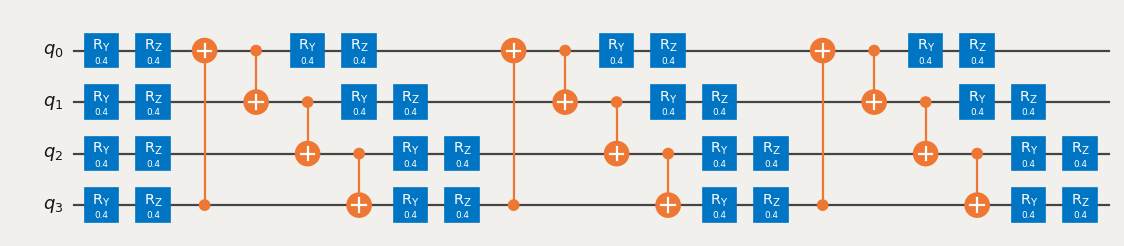
from qiskit.circuit.library import efficient_su2

circuit = efficient_su2(num_qubits=4, entanglement="circular")
circuit.assign_parameters([0.4] * len(circuit.parameters), inplace=True)
circuit.draw("mpl", scale=0.8)

Tukuyin ang isang observable

from qiskit.quantum_info import SparsePauliOp

observable = SparsePauliOp(["ZZII", "IZZI", "-IIZZ", "XIXI", "ZIZZ", "IXIX"])

Hakbang 2: Optimize

Tukuyin ang isang backend

Maaari kang magbigay ng alinman sa fake backend o hardware backend mula sa Qiskit Runtime.

from qiskit_ibm_runtime.fake_provider import FakeManilaV2

backend = FakeManilaV2()

I-transpile ang circuit, i-visualize ang mga swap, at tandaan ang depth

Pumipili tayo ng layout na nangangailangan ng dalawang swap upang isagawa ang mga gate sa pagitan ng qubits 3 at 0 at isa pang dalawang swap upang ibalik ang mga qubit sa kanilang inisyal na posisyon.

from qiskit.transpiler import generate_preset_pass_manager

pass_manager = generate_preset_pass_manager(
    optimization_level=1, backend=backend, initial_layout=[0, 1, 2, 3]
)

transpiled_qc = pass_manager.run(circuit)
print(f"Transpiled circuit depth: {transpiled_qc.depth(lambda x: len(x.qubits) >= 2)}")

Transpiled circuit depth: 30

transpiled_qc.draw("mpl", scale=0.4, idle_wires=False, fold=-1)

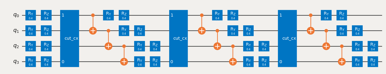
Palitan ang mga distant gate ng TwoQubitQPDGates sa pamamagitan ng pagtukoy ng kanilang mga indices

Ang cut_gates ay papalitan ang mga gate sa tinukoy na mga index ng TwoQubitQPDGates at magbabalik din ng listahan ng mga QPDBasis instance -- isa para sa bawat gate decomposition.

from qiskit_addon_cutting import cut_gates

# Find the indices of the distant gates
cut_indices = [
    i
    for i, instruction in enumerate(circuit.data)
    if {circuit.find_bit(q)[0] for q in instruction.qubits} == {0, 3}
]

# Decompose distant CNOTs into TwoQubitQPDGate instances
qpd_circuit, bases = cut_gates(circuit, cut_indices)

qpd_circuit.draw("mpl", scale=0.8)

Bumuo ng mga subexperiment na patatakbuhin sa backend

Ang generate_cutting_experiments ay tumatanggap ng circuit na naglalaman ng mga TwoQubitQPDGate instance at observables bilang PauliList.

Upang i-simulate ang expectation value ng full-sized na circuit, maraming subexperiment ang nabubuo mula sa joint quasiprobability distribution ng mga decomposed na gate at pagkatapos ay isinasagawa sa isa o higit pang backend. Ang bilang ng mga sample na kinukuha mula sa distribution ay kinokontrol ng num_samples, at isang combined coefficient ang ibinibigay para sa bawat unique sample. Para sa karagdagang impormasyon kung paano kinakalkula ang mga coefficient, sumangguni sa explanatory material.

Tandaan: Ang observables kwarg sa generate_cutting_experiments ay may type na PauliList. Ang mga observable term coefficient at phase ay binabalewala sa panahon ng decomposition ng problema at execution ng mga subexperiment. Maaari silang ilapat muli sa panahon ng reconstruction ng expectation value.

import numpy as np
from qiskit_addon_cutting import generate_cutting_experiments

# Generate the subexperiments and sampling coefficients
subexperiments, coefficients = generate_cutting_experiments(
    circuits=qpd_circuit, observables=observable.paulis, num_samples=np.inf
)

Kalkulahin ang sampling overhead para sa napiling mga cut

Dito, pinuputol natin ang tatlong CNOT gate, na nagreresulta sa sampling overhead na $9^3$.

Para sa higit pa tungkol sa sampling overhead na nakukuha mula sa circuit cutting, sumangguni sa explanatory material.

print(f"Sampling overhead: {np.prod([basis.overhead for basis in bases])}")

Sampling overhead: 729.0

Ipakita na ang mga QPD subexperiment ay magiging mas shallow pagkatapos putulin ang mga distant gate

Narito ang halimbawa ng isang arbitraryong napiling subexperiment na nabuo mula sa QPD circuit. Ang depth nito ay nabawasan nang higit sa kalahati. Marami sa mga probabilistic subexperiment na ito ang dapat mabuo at masuri upang ma-reconstruct ang isang expectation value ng mas malalim na circuit.

# Transpile the decomposed circuit to the same layout
transpiled_qpd_circuit = pass_manager.run(subexperiments[100])

print(
    f"Original circuit depth after transpile: {transpiled_qc.depth(lambda x: len(x.qubits) >= 2)}"
)
print(
    f"QPD subexperiment depth after transpile: {transpiled_qpd_circuit.depth(lambda x: len(x.qubits) >= 2)}"
)
transpiled_qpd_circuit.draw("mpl", scale=0.8, idle_wires=False, fold=-1)

Original circuit depth after transpile: 30
QPD subexperiment depth after transpile: 7

Ihanda ang mga subexperiment para sa backend

# Transpile the subeperiments to the backend's instruction set architecture (ISA)
isa_subexperiments = pass_manager.run(subexperiments)

Hakbang 3: Execute

Patakbuhin ang mga subexperiment gamit ang Qiskit Runtime Sampler primitive

from qiskit_ibm_runtime import SamplerV2

# Set up the Qiskit Runtime Sampler primitive.  For a fake backend, this will use a local simulator.
sampler = SamplerV2(backend)

# Submit the subexperiments
job = sampler.run(isa_subexperiments)

# Retrieve the results
results = job.result()

Hakbang 4: Post-process

I-reconstruct ang expectation value

I-reconstruct ang expectation values para sa bawat observable term at pagsamahin ang mga ito upang ma-reconstruct ang expectation value para sa orihinal na observable.

from qiskit_addon_cutting import reconstruct_expectation_values

reconstructed_expval_terms = reconstruct_expectation_values(
    results,
    coefficients,
    observable.paulis,
)
# Reconstruct final expectation value
reconstructed_expval = np.dot(reconstructed_expval_terms, observable.coeffs)

Ikumpara ang reconstructed expectation value sa exact expectation value mula sa orihinal na circuit at observable

from qiskit_aer.primitives import EstimatorV2

estimator = EstimatorV2()
exact_expval = estimator.run([(circuit, observable)]).result()[0].data.evs
print(f"Reconstructed expectation value: {np.real(np.round(reconstructed_expval, 8))}")
print(f"Exact expectation value: {np.round(exact_expval, 8)}")
print(f"Error in estimation: {np.real(np.round(reconstructed_expval-exact_expval, 8))}")
print(
    f"Relative error in estimation: {np.real(np.round((reconstructed_expval-exact_expval) / exact_expval, 8))}"
)

Reconstructed expectation value: 0.44018555
Exact expectation value: 0.50497603
Error in estimation: -0.06479049
Relative error in estimation: -0.12830408