Utility-scale na pagbabawas ng error gamit ang probabilistic error amplification
Tinatayang paggamit: 14 minuto sa isang Heron r3 na processor (TANDAAN: Tantya lamang ito. Maaaring mag-iba ang iyong aktwal na oras ng pagpapatakbo.)
Mga layunin sa pag-aaral
Pagkatapos ng tutorial na ito, dapat maunawaan ng mga gumagamit ang:
- Ang teorya sa likod ng zero-noise extrapolation (ZNE), ang iba't ibang paraan ng pag-amplify ng ingay, at kung bakit mas pinipili ang probabilistic error amplification (PEA) para sa mga utility-scale na eksperimento.
- Kung paano ipatupad ang ZNE gamit ang PEA sa praktis gamit ang Qiskit.
Mga Kinakailangan
Iminumungkahi naming maging pamilyar ang mga gumagamit sa mga sumusunod na paksa bago dumaan sa tutorial na ito:
- Ang aralin sa Error mitigation ng kursong Utility-scale quantum computing para sa pangunahing kaalaman sa paggamit ng error mitigation sa Qiskit.
- Ang aralin sa Utility-I ng kursong Utility-scale quantum computing para sa karagdagang impormasyon tungkol sa utility-scale na eksperimentong ginagamit bilang halimbawa sa tutorial na ito.
Panimula
Ipinapakita ng tutorial na ito kung paano magsagawa ng utility-scale na eksperimento sa pagbabawas ng error gamit ang Qiskit Runtime, sa pamamagitan ng isang eksperimental na bersyon ng zero-noise extrapolation (ZNE) kasama ang probabilistic error amplification (PEA).
 Sanggunian: Y. Kim et al. Evidence for the utility of quantum computing before fault tolerance. Nature 618.7965 (2023)
Zero-noise extrapolation (ZNE)
Ang zero-noise extrapolation (ZNE) ay isang teknik sa pagbabawas ng error na nag-aalis ng mga epekto ng hindi kilalang ingay sa panahon ng pagpapatakbo ng circuit, na maaaring i-scale sa isang kilalang paraan.
Ipinapalagay nito na ang mga inaasahang halaga ay nag-iiba ayon sa ingay sa pamamagitan ng isang kilalang function
kung saan ang ay nagpaparameter ng lakas ng ingay at maaaring palakasin.
Maaari nating ipatupad ang ZNE sa pamamagitan ng mga sumusunod na hakbang:
- Palakihin ang ingay ng circuit para sa ilang noise factor na
- Patakbuhin ang bawat noise-amplified na circuit upang masukat ang
- I-extrapolate pabalik sa zero-noise limit na

Pagpapalaki ng ingay para sa ZNE
Ang pangunahing hamon sa matagumpay na pagpapatupad ng ZNE ay ang pagkakaroon ng tumpak na modelo para sa ingay sa inaasahang halaga at ang pagpapalaki ng ingay sa isang kilalang paraan.
Mayroong tatlong karaniwang paraan ng pagpapatupad ng error amplification para sa ZNE.
| Pulse stretching | Gate folding | Probabilistic error amplification |
|---|---|---|
| Scale pulse duration via calibration | Repeat gates in identity cycles | Add noise via sampling Pauli channels |
 |  |  |
| Kandala et al. Nature (2019) | Shultz et al. PRA (2022) | Li & Benjamin PRX (2017) |
| Para sa mga utility-scale na eksperimento, ang probabilistic error amplification (PEA) ang pinaka-angkop. |
- Ipinapalagay ng pulse stretching na ang ingay ng gate ay proporsyonal sa tagal, na kadalasang hindi totoo. Mahal din ang kalibrasyon.
- Ang gate folding ay nangangailangan ng malalaking stretch factor na lubos na nagpapalimit sa lalim ng mga circuit na maaaring patakbuhin.
- Ang PEA ay maaaring ilapat sa anumang circuit na maaaring patakbuhin na may katutubong noise factor () ngunit nangangailangan ng pag-aaral ng noise model.
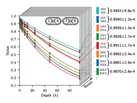
Pag-aaral ng noise model para sa PEA
Ipinapalagay ng PEA ang parehong layer-based na noise model katulad ng probabilistic error cancellation (PEC); gayunpaman, iniiwasan nito ang sampling overhead na lumalago nang exponential kasabay ng ingay ng circuit.
| Hakbang 1 | Hakbang 2 | Hakbang 3 |
|---|---|---|
| Pauli twirl layers of two-qubit gates | Repeat identity pairs of layers and learn the noise | Derive a fidelity (error for each noise channel) |
 | 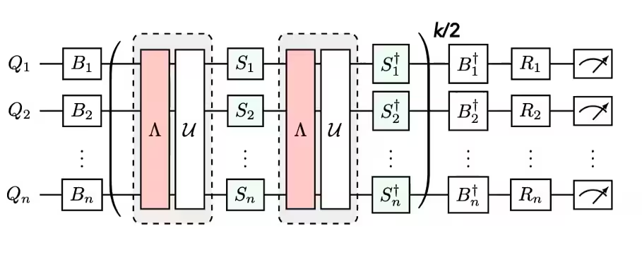 |  |
Sanggunian: E. van den Berg, Z. Minev, A. Kandala, and K. Temme, Probabilistic error cancellation with sparse Pauli-Lindblad models on noisy quantum processors arXiv:2201.09866
Mga Kinakailangan
Bago simulan ang tutorial na ito, tiyaking naka-install ang mga sumusunod:
- Qiskit SDK v2.0 o mas bago, na may suporta para sa visualization
- Qiskit Runtime v0.22 o mas bago (
pip install qiskit-ibm-runtime)
Setup
Sa cell sa ibaba, nag-i-import kami ng mga kaugnay na pakete at gumagawa ng ilang helper function upang buuin ang mga circuit para sa Trotterized time evolution ng isang dalawang-dimensyonal na transverse-field Ising model na sumusunod sa topology ng backend.
# Added by doQumentation — required packages for this notebook
!pip install -q matplotlib numpy qiskit qiskit-ibm-runtime rustworkx
from __future__ import annotations
from collections.abc import Sequence
from collections import defaultdict
import numpy as np
import rustworkx
import matplotlib.pyplot as plt

from qiskit.circuit import QuantumCircuit, Parameter
from qiskit.circuit.library import CXGate, CZGate, ECRGate
from qiskit.providers import Backend
from qiskit.visualization import plot_error_map
from qiskit.transpiler.preset_passmanagers import generate_preset_pass_manager
from qiskit.quantum_info import SparsePauliOp
from qiskit.primitives import PubResult

from qiskit_ibm_runtime import QiskitRuntimeService
from qiskit_ibm_runtime import EstimatorV2 as Estimator

"""Trotter circuit generation"""

def remove_qubit_couplings(
    couplings: Sequence[tuple[int, int]], qubits: Sequence[int] | None = None
) -> list[tuple[int, int]]:
    """Remove qubits from a coupling list.

    Args:
        couplings: A sequence of qubit couplings.
        qubits: Optional, the qubits to remove.

    Returns:
        The input couplings with the specified qubits removed.
    """
    if qubits is None:
        return couplings
    qubits = set(qubits)
    return [edge for edge in couplings if not qubits.intersection(edge)]

def coupling_qubits(
    *couplings: Sequence[tuple[int, int]],
    allowed_qubits: Sequence[int] | None = None,
) -> list[int]:
    """Return a sorted list of all qubits involved in one or more couplings lists.

    Args:
        couplings: one or more coupling lists.
        allowed_qubits: Optional, the allowed qubits to include. If None all
            qubits are allowed.

    Returns:
        The intersection of all qubits in the couplings and the allowed qubits.
    """
    qubits = set()
    for edges in couplings:
        for edge in edges:
            qubits.update(edge)
    if allowed_qubits is not None:
        qubits = qubits.intersection(allowed_qubits)
    return list(qubits)

def construct_layer_couplings(
    backend: Backend,
) -> list[list[tuple[int, int]]]:
    """Separate a coupling map into disjoint 2-qubit gate layers.

    Args:
        backend: A backend to construct layer couplings for.

    Returns:
        A list of disjoint layers of directed couplings for the input coupling map.
    """
    coupling_graph = backend.coupling_map.graph.to_undirected(
        multigraph=False
    )
    edge_coloring = rustworkx.graph_bipartite_edge_color(coupling_graph)

    layers = defaultdict(list)
    for edge_idx, color in edge_coloring.items():
        layers[color].append(
            coupling_graph.get_edge_endpoints_by_index(edge_idx)
        )
    layers = [sorted(layers[i]) for i in sorted(layers.keys())]

    return layers

def entangling_layer(
    gate_2q: str,
    couplings: Sequence[tuple[int, int]],
    qubits: Sequence[int] | None = None,
) -> QuantumCircuit:
    """Generating a entangling layer for the specified couplings.

    This corresponds to a Trotter layer for a ZZ Ising term with angle Pi/2.

    Args:
        gate_2q: The 2-qubit basis gate for the layer, should be "cx", "cz", or "ecr".
        couplings: A sequence of qubit couplings to add CX gates to.
        qubits: Optional, the physical qubits for the layer. Any couplings involving
            qubits not in this list will be removed. If None the range up to the largest
            qubit in the couplings will be used.

    Returns:
        The QuantumCircuit for the entangling layer.
    """
    # Get qubits and convert to set to order
    if qubits is None:
        qubits = range(1 + max(coupling_qubits(couplings)))
    qubits = set(qubits)

    # Mapping of physical qubit to virtual qubit
    qubit_mapping = {q: i for i, q in enumerate(qubits)}

    # Convert couplings to indices for virtual qubits
    indices = [
        [qubit_mapping[i] for i in edge]
        for edge in couplings
        if qubits.issuperset(edge)
    ]

    # Layer circuit on virtual qubits
    circuit = QuantumCircuit(len(qubits))

    # Get 2-qubit basis gate and pre and post rotation circuits
    gate2q = None
    pre = QuantumCircuit(2)
    post = QuantumCircuit(2)

    if gate_2q == "cx":
        gate2q = CXGate()
        # Pre-rotation
        pre.sdg(0)
        pre.z(1)
        pre.sx(1)
        pre.s(1)
        # Post-rotation
        post.sdg(1)
        post.sxdg(1)
        post.s(1)
    elif gate_2q == "ecr":
        gate2q = ECRGate()
        # Pre-rotation
        pre.z(0)
        pre.s(1)
        pre.sx(1)
        pre.s(1)
        # Post-rotation
        post.x(0)
        post.sdg(1)
        post.sxdg(1)
        post.s(1)
    elif gate_2q == "cz":
        gate2q = CZGate()
        # Identity pre-rotation
        # Post-rotation
        post.sdg([0, 1])
    else:
        raise ValueError(
            f"Invalid 2-qubit basis gate {gate_2q}, should be 'cx', 'cz', or 'ecr'"
        )

    # Add 1Q pre-rotations
    for inds in indices:
        circuit.compose(pre, qubits=inds, inplace=True)

    # Use barriers around 2-qubit basis gate to specify a layer for PEA noise learning
    circuit.barrier()
    for inds in indices:
        circuit.append(gate2q, (inds[0], inds[1]))
    circuit.barrier()

    # Add 1Q post-rotations after barrier
    for inds in indices:
        circuit.compose(post, qubits=inds, inplace=True)

    # Add physical qubits as metadata
    circuit.metadata["physical_qubits"] = tuple(qubits)

    return circuit

def trotter_circuit(
    theta: Parameter | float,
    layer_couplings: Sequence[Sequence[tuple[int, int]]],
    num_steps: int,
    gate_2q: str | None = "cx",
    backend: Backend | None = None,
    qubits: Sequence[int] | None = None,
) -> QuantumCircuit:
    """Generate a Trotter circuit for the 2D Ising

    Args:
        theta: The angle parameter for X.
        layer_couplings: A list of couplings for each entangling layer.
        num_steps: the number of Trotter steps.
        gate_2q: The 2-qubit basis gate to use in entangling layers.
            Can be "cx", "cz", "ecr", or None if a backend is provided.
        backend: A backend to get the 2-qubit basis gate from, if provided
            will override the basis_gate field.
        qubits: Optional, the allowed physical qubits to truncate the
            couplings to. If None the range up to the largest
            qubit in the couplings will be used.

    Returns:
        The Trotter circuit.
    """
    if backend is not None:
        try:
            basis_gates = backend.configuration().basis_gates
        except AttributeError:
            basis_gates = backend.basis_gates
        for gate in ["cx", "cz", "ecr"]:
            if gate in basis_gates:
                gate_2q = gate
                break

    # If no qubits, get the largest qubit from all layers and
    # specify the range so the same one is used for all layers.
    if qubits is None:
        qubits = range(1 + max(coupling_qubits(layer_couplings)))

    # Generate the entangling layers
    layers = [
        entangling_layer(gate_2q, couplings, qubits=qubits)
        for couplings in layer_couplings
    ]

    # Construct the circuit for a single Trotter step
    num_qubits = len(qubits)
    trotter_step = QuantumCircuit(num_qubits)
    trotter_step.rx(theta, range(num_qubits))
    for layer in layers:
        trotter_step.compose(layer, range(num_qubits), inplace=True)

    # Construct the circuit for the specified number of Trotter steps
    circuit = QuantumCircuit(num_qubits)
    for _ in range(num_steps):
        circuit.rx(theta, range(num_qubits))
        for layer in layers:
            circuit.compose(layer, range(num_qubits), inplace=True)

    circuit.metadata["physical_qubits"] = tuple(qubits)
    return circuit

"""Result visualization functions"""

def plot_trotter_results(
    pub_result: PubResult,
    angles: Sequence[float],
    plot_noise_factors: Sequence[float] | None = None,
    plot_extrapolator: Sequence[str] | None = None,
    exact: np.ndarray = None,
    close: bool = True,
):
    """Plot average magnetization from ZNE result data.
    Args:
        pub_result: The Estimator PubResult for the PEA experiment.
        angles: The Rx angle values for the experiment.
        plot_raw: If provided plot the unextrapolated data for the noise factors.
        plot_extrapolator: If provided plot all extrapolators, if False only plot
            the Automatic method.
        exact: Optional, the exact values to include in the plot. Should be a 1D
            array-like where the values represent exact magnetization.
        close: Close the Matplotlib figure before returning.
    Returns:
        The figure.
    """
    data = pub_result.data

    evs = data.evs
    num_qubits = evs.shape[0]
    num_params = evs.shape[1]
    angles = np.asarray(angles).ravel()
    if angles.shape != (num_params,):
        raise ValueError(
            f"Incorrect number of angles for input data {angles.size} != {num_params}"
        )

    # Take average magnetization of qubits and its standard error
    x_vals = angles / np.pi
    y_vals = np.mean(evs, axis=0)
    y_errs = np.std(evs, axis=0) / np.sqrt(num_qubits)

    fig, _ = plt.subplots(1, 1)

    # Plot auto method
    plt.errorbar(x_vals, y_vals, y_errs, fmt="o-", label="ZNE (automatic)")

    # Plot individual extrapolator results
    if plot_extrapolator:
        y_vals_extrap = np.mean(data.evs_extrapolated, axis=0)
        y_errs_extrap = np.std(data.evs_extrapolated, axis=0) / np.sqrt(
            num_qubits
        )
        for i, extrap in enumerate(plot_extrapolator):
            plt.errorbar(
                x_vals,
                y_vals_extrap[:, i, 0],
                y_errs_extrap[:, i, 0],
                fmt="s-.",
                alpha=0.5,
                label=f"ZNE ({extrap})",
            )

    # Plot raw results
    if plot_noise_factors:
        y_vals_raw = np.mean(data.evs_noise_factors, axis=0)
        y_errs_raw = np.std(data.evs_noise_factors, axis=0) / np.sqrt(
            num_qubits
        )
        for i, nf in enumerate(plot_noise_factors):
            plt.errorbar(
                x_vals,
                y_vals_raw[:, i],
                y_errs_raw[:, i],
                fmt="d:",
                alpha=0.5,
                label=f"Raw (nf={nf:.1f})",
            )

    # Plot exact data
    if exact is not None:
        plt.plot(x_vals, exact, "--", color="black", alpha=0.5, label="Exact")

    plt.ylim(-0.1, 1.2)
    plt.xlabel("θ/π")
    plt.ylabel(r"$\overline{\langle Z \rangle}$")
    plt.legend()
    plt.title(
        f"Error Mitigated Average Magnetization for Rx(θ) [{num_qubits}-qubit]"
    )
    if close:
        plt.close(fig)
    return fig

def plot_qubit_zne_data(
    pub_result: PubResult,
    angles: Sequence[float],
    qubit: int,
    noise_factors: Sequence[float],
    extrapolator: Sequence[str] | None = None,
    extrapolated_noise_factors: Sequence[float] | None = None,
    num_cols: int | None = None,
    close: bool = True,
):
    """Plot ZNE extrapolation data for specific virtual qubit
    Args:
        pub_result: The Estimator PubResult for the PEA experiment.
        angles: The Rx theta angles used for the experiment.
        qubit: The virtual qubit index to plot.
        noise_factors: the raw noise factors.
        extrapolator: The extrapolator metadata for multiple extrapolators.
        extrapolated_noise_factors: The noise factors used for extrapolation.
        num_cols: The number of columns for the generated subplots.
        close: Close the Matplotlib figure before returning.
    Returns:
        The Matplotlib figure.
    """
    data = pub_result.data

    evs_auto = data.evs[qubit]
    stds_auto = data.stds[qubit]
    evs_extrap = data.evs_extrapolated[qubit]
    stds_extrap = data.stds_extrapolated[qubit]
    evs_raw = data.evs_noise_factors[qubit]
    stds_raw = data.stds_noise_factors[qubit]

    num_params = evs_auto.shape[0]
    angles = np.asarray(angles).ravel()
    if angles.shape != (num_params,):
        raise ValueError(
            f"Incorrect number of angles for input data {angles.size} != {num_params}"
        )

    # Make a square subplot
    num_cols = num_cols or int(np.ceil(np.sqrt(num_params)))
    num_rows = int(np.ceil(num_params / num_cols))
    fig, axes = plt.subplots(
        num_rows, num_cols, sharex=True, sharey=True, figsize=(12, 5)
    )
    fig.suptitle(f"ZNE data for virtual qubit {qubit}")

    for pidx, ax in zip(range(num_params), axes.flat):
        # Plot auto extrapolated
        ax.errorbar(
            0,
            evs_auto[pidx],
            stds_auto[pidx],
            fmt="o",
            label="PEA (automatic)",
        )

        # Plot extrapolators
        if (
            extrapolator is not None
            and extrapolated_noise_factors is not None
        ):
            for i, method in enumerate(extrapolator):
                ax.errorbar(
                    extrapolated_noise_factors,
                    evs_extrap[pidx, i],
                    stds_extrap[pidx, i],
                    fmt="-",
                    alpha=0.5,
                    label=f"PEA ({method})",
                )

        # Plot raw
        ax.errorbar(
            noise_factors, evs_raw[pidx], stds_raw[pidx], fmt="d", label="Raw"
        )

        ax.set_yticks([0, 0.5, 1, 1.5, 2])
        ax.set_ylim(0, max(1, 1.1 * max(evs_auto)))

        ax.set_xticks([0, *noise_factors])
        ax.set_title(f"θ/π = {angles[pidx]/np.pi:.2f}")
        if pidx == 0:
            ax.set_ylabel(r"$\langle Z_{" + str(qubit) + r"} \rangle$")
        if pidx == num_params - 1:
            ax.set_xlabel("Noise Factor")
            ax.legend()
    plt.tight_layout()
    if close:
        plt.close(fig)
    return fig
Halimbawa sa maliit na sukat gamit ang simulator
Lalaktawan namin ang hakbang na ito dahil hindi sinusuportahan ang runtime error mitigation sa mga simulator.
Halimbawa sa malaking sukat sa hardware
Hakbang 1: I-map ang mga klasikal na input sa isang quantum na problema
Lumikha ng parameterized Ising model circuit
Magtatag ng backend
Una, pumili ng backend na pagpapatakbuhin. Ang demonstrasyong ito ay tumatakbo sa isang 127-qubit na backend, ngunit maaari mo itong baguhin para sa anumang backend na available sa iyo.
service = QiskitRuntimeService()
backend = service.least_busy(
    operational=True, simulator=False, min_num_qubits=127
)
backend
<IBMBackend('ibm_fez')>
Tukuyin ang mga entangling layer coupling
Upang maipatupad ang Trotterized Ising simulation, tukuyin ang tatlong layer ng two-qubit gate coupling para sa device, na uulitin sa bawat Trotter step. Tinutukoy ng mga ito ang tatlong twirled layer na kailangang matutunan ang ingay upang maipatupad ang mitigation.
layer_couplings = construct_layer_couplings(backend)
for i, layer in enumerate(layer_couplings):
    print(f"Layer {i}:\n{layer}\n")
Layer 0:
[(2, 3), (4, 5), (6, 7), (8, 9), (10, 11), (12, 13), (14, 15), (16, 23), (18, 31), (19, 35), (20, 21), (25, 37), (26, 27), (28, 29), (33, 39), (36, 41), (38, 49), (42, 43), (45, 46), (47, 57), (51, 52), (53, 54), (56, 63), (58, 71), (59, 75), (61, 62), (64, 65), (66, 67), (68, 69), (72, 73), (76, 81), (79, 93), (82, 83), (84, 85), (86, 87), (88, 89), (91, 98), (94, 95), (97, 107), (99, 115), (100, 101), (102, 103), (105, 117), (108, 109), (110, 111), (113, 114), (116, 121), (118, 129), (123, 136), (124, 125), (126, 127), (130, 131), (132, 133), (135, 139), (138, 151), (142, 143), (144, 145), (146, 147), (152, 153), (154, 155)]

Layer 1:
[(0, 1), (3, 16), (5, 6), (7, 8), (11, 18), (13, 14), (17, 27), (21, 22), (23, 24), (25, 26), (29, 38), (30, 31), (32, 33), (34, 35), (39, 53), (41, 42), (43, 56), (44, 45), (47, 48), (49, 50), (51, 58), (54, 55), (57, 67), (60, 61), (62, 63), (65, 66), (69, 78), (70, 71), (73, 79), (74, 75), (77, 85), (80, 81), (83, 84), (87, 97), (89, 90), (91, 92), (93, 94), (96, 103), (101, 116), (104, 105), (106, 107), (109, 118), (111, 112), (113, 119), (114, 115), (117, 125), (121, 122), (123, 124), (127, 137), (128, 129), (131, 138), (133, 134), (136, 143), (139, 155), (140, 141), (145, 146), (147, 148), (149, 150), (151, 152)]

Layer 2:
[(1, 2), (3, 4), (7, 17), (9, 10), (11, 12), (15, 19), (21, 36), (22, 23), (24, 25), (27, 28), (29, 30), (31, 32), (33, 34), (37, 45), (40, 41), (43, 44), (46, 47), (48, 49), (50, 51), (52, 53), (55, 59), (61, 76), (63, 64), (65, 77), (67, 68), (69, 70), (71, 72), (73, 74), (78, 89), (81, 82), (83, 96), (85, 86), (87, 88), (90, 91), (92, 93), (95, 99), (98, 111), (101, 102), (103, 104), (105, 106), (107, 108), (109, 110), (112, 113), (119, 133), (120, 121), (122, 123), (125, 126), (127, 128), (129, 130), (131, 132), (134, 135), (137, 147), (141, 142), (143, 144), (148, 149), (150, 151), (153, 154)]
Alisin ang mga masamang qubit
Tingnan ang coupling map ng backend at alamin kung may mga qubit na may mataas na error na koneksyon. Alisin ang mga "masamang" qubit na ito mula sa iyong eksperimento.
# Plot gate error map
# NOTE: These can change over time, so your results may look different
plot_error_map(backend)
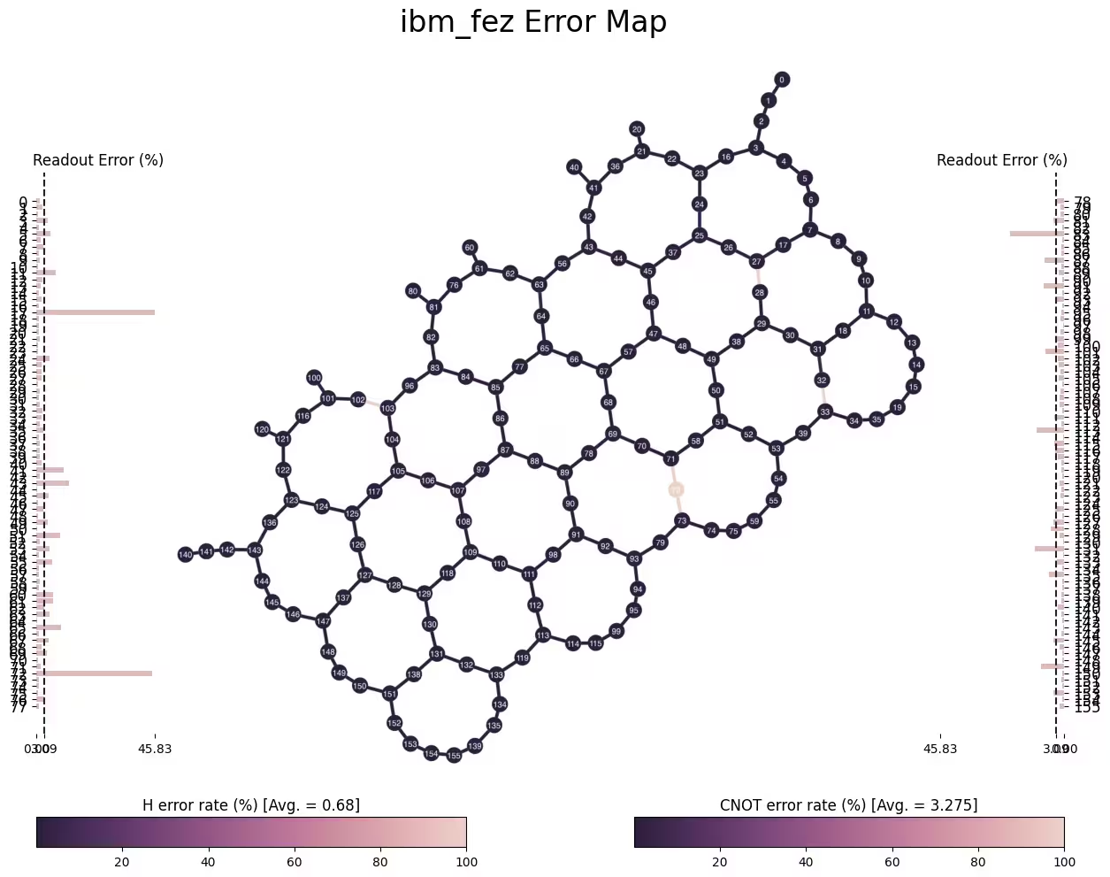
bad_qubits = {
    32,
    33,
    71,
    72,
    73,
    102,
    103,
}  # qubits removed based on high coupling error (1.00)
good_qubits = list(set(range(backend.num_qubits)).difference(bad_qubits))
print("Physical qubits:\n", good_qubits)
Physical qubits:
 [0, 1, 2, 3, 4, 5, 6, 7, 8, 9, 10, 11, 12, 13, 14, 15, 16, 17, 18, 19, 20, 21, 22, 23, 24, 25, 26, 27, 28, 29, 30, 31, 34, 35, 36, 37, 38, 39, 40, 41, 42, 43, 44, 45, 46, 47, 48, 49, 50, 51, 52, 53, 54, 55, 56, 57, 58, 59, 60, 61, 62, 63, 64, 65, 66, 67, 68, 69, 70, 74, 75, 76, 77, 78, 79, 80, 81, 82, 83, 84, 85, 86, 87, 88, 89, 90, 91, 92, 93, 94, 95, 96, 97, 98, 99, 100, 101, 104, 105, 106, 107, 108, 109, 110, 111, 112, 113, 114, 115, 116, 117, 118, 119, 120, 121, 122, 123, 124, 125, 126, 127, 128, 129, 130, 131, 132, 133, 134, 135, 136, 137, 138, 139, 140, 141, 142, 143, 144, 145, 146, 147, 148, 149, 150, 151, 152, 153, 154, 155]
Pangunahing pagbuo ng Trotter circuit
num_steps = 6
theta = Parameter("theta")
circuit = trotter_circuit(
    theta, layer_couplings, num_steps, qubits=good_qubits, backend=backend
)
Lumikha ng listahan ng mga parameter value na itatakda sa ibang pagkakataon
num_params = 12

# 12 parameter values for Rx between [0, pi/2].
# Reshape to outer product broadcast with observables
parameter_values = np.linspace(0, np.pi / 2, num_params).reshape(
    (num_params, 1)
)
num_params = parameter_values.size
Hakbang 2: I-optimize ang problema para sa pagpapatakbo sa quantum hardware
ISA circuit
Bago patakbuhin ang circuit sa hardware, i-optimize ito para sa pagpapatakbo sa hardware. Ang prosesong ito ay kinabibilangan ng ilang hakbang:
- Pumili ng qubit layout na nag-map ng mga virtual qubit ng iyong circuit sa mga pisikal na qubit sa hardware.
- Maglagay ng mga swap gate kung kinakailangan upang mailagay ang mga interaksyon sa pagitan ng mga qubit na hindi konektado.
- I-translate ang mga gate sa aming circuit sa mga tagubilin ng Instruction Set Architecture (ISA) na maaaring direktang isagawa sa hardware.
- Magsagawa ng mga pag-optimize ng circuit upang mabawasan ang lalim at bilang ng gate ng circuit.
Bagaman ang transpiler na built-in sa Qiskit ay kayang isagawa ang lahat ng hakbang na ito, ipinapakita ng tutorial na ito ang pagbuo ng utility-scale Trotter circuit mula sa simula. Piliin ang mga magagandang pisikal na qubit at tukuyin ang mga entangling layer sa mga konektadong pares ng qubit mula sa mga piling qubit na iyon. Gayunpaman, kailangan pa ring i-translate ang mga hindi ISA na gate sa circuit at samantalahin ang anumang pag-optimize ng circuit na inaalok ng transpiler.
I-transpile ang iyong circuit para sa piniling backend sa pamamagitan ng paglikha ng pass manager at pagpapatakbo ng pass manager sa circuit. Gayundin, itakda ang paunang layout ng circuit sa nang napiling good_qubits. Ang isang madaling paraan upang lumikha ng pass manager ay ang paggamit ng function na generate_preset_pass_manager. Tingnan ang Transpile with pass managers para sa mas detalyadong paliwanag ng pag-transpile gamit ang mga pass manager.
pm = generate_preset_pass_manager(
    backend=backend,
    initial_layout=good_qubits,
    layout_method="trivial",
    optimization_level=1,
)

isa_circuit = pm.run(circuit)
Mga ISA observable
Susunod, lumikha ng lahat ng weight-1 na observable para sa bawat virtual qubit sa pamamagitan ng pagdadagdag ng kinakailangang bilang ng mga term.
observables = []
num_qubits = len(good_qubits)
for q in range(num_qubits):
    observables.append(
        SparsePauliOp("I" * (num_qubits - q - 1) + "Z" + "I" * q)
    )
Ini-map ng proseso ng transpilation ang mga virtual qubit ng iyong circuit sa mga pisikal na qubit sa hardware. Ang impormasyon tungkol sa layout ng qubit ay nakaimbak sa katangiang layout ng transpiled circuit. Ang iyong observable ay tinukoy din sa mga tuntunin ng mga virtual qubit, kaya kailangan mong ilapat ang layout na ito sa observable. Ginagawa ito gamit ang paraang apply_layout ng SparsePauliOp.
Pansinin na ang bawat observable ay nakabalot sa isang listahan sa sumusunod na bloke ng code. Ginagawa ito upang i-broadcast kasama ang mga parameter value upang ang bawat qubit observable ay masukat para sa bawat theta value. Hanapin ang mga panuntunan sa broadcasting para sa mga primitive sa dokumentasyon ng mga primitive.
isa_observables = [
    [obs.apply_layout(layout=isa_circuit.layout)] for obs in observables
]
Hakbang 3: Isagawa gamit ang Qiskit primitives
pub = (isa_circuit, isa_observables, parameter_values)
I-configure ang mga opsyon ng Estimator
Susunod, i-configure ang mga opsyon ng Estimator na kailangan para sa pagpapatakbo ng eksperimento sa mitigation. Kasama rito ang mga opsyon para sa noise learning ng mga entangling layer, at para sa ZNE extrapolation.
Ginagamit namin ang sumusunod na configuration:
# Experiment options
num_randomizations = 700
num_randomizations_learning = 40
max_batch_circuits = 3 * num_params
shots_per_randomization = 64
learning_pair_depths = [0, 1, 2, 4, 6, 12, 24]
noise_factors = [1, 1.3, 1.6]
extrapolated_noise_factors = np.linspace(0, max(noise_factors), 20)

# Base option formatting
options = {
    # Builtin resilience settings for ZNE
    "resilience": {
        "measure_mitigation": True,
        "zne_mitigation": True,
        # TREX noise learning configuration
        "measure_noise_learning": {
            "num_randomizations": num_randomizations_learning,
            "shots_per_randomization": 1024,
        },
        # PEA noise model configuration
        "layer_noise_learning": {
            "max_layers_to_learn": 3,
            "layer_pair_depths": learning_pair_depths,
            "shots_per_randomization": shots_per_randomization,
            "num_randomizations": num_randomizations_learning,
        },
        "zne": {
            "amplifier": "pea",
            "noise_factors": noise_factors,
            "extrapolator": ("exponential", "linear"),
            "extrapolated_noise_factors": extrapolated_noise_factors.tolist(),
        },
    },
    # Randomization configuration
    "twirling": {
        "num_randomizations": num_randomizations,
        "shots_per_randomization": shots_per_randomization,
        "strategy": "active-circuit",
    },
    # Optional Dynamical Decoupling (DD)
    "dynamical_decoupling": {"enable": True, "sequence_type": "XY4"},
    # Job tag
    "environment": {"job_tags": ["TUT_PEA"]},
}
Paliwanag ng mga opsyon ng ZNE
Ang sumusunod ay nagbibigay ng detalye tungkol sa mga karagdagang opsyon sa experimental branch. Tandaan na ang mga opsyon at pangalan na ito ay hindi pa pinal, at lahat ng narito ay maaaring magbago bago ang opisyal na release.
- amplifier: Ang paraan na gagamitin sa pag-amplify ng noise patungo sa mga nilalayon na noise factor.
Ang mga pinahintulutang halaga ay
"gate_folding", na nag-a-amplify sa pamamagitan ng pag-uulit ng two-qubit basis gates, at"pea", na nag-a-amplify sa pamamagitan ng probabilistic sampling matapos matutunan ang Pauli-twirled na noise model para sa mga layer ng twirled two-qubit basis gates. Ang mga karagdagang opsyon ay"gate_folding_front"at"gate_folding_back", na ipinaliwanag sa API documentation. - extrapolated_noise_factors: Tumukoy ng isa o higit pang halaga ng noise factor kung saan susuriin ang mga extrapolated na modelo. Kung isang sequence ng mga halaga ang ibinigay, ang mga ibinalik na resulta ay magiging array-valued na may tinukoy na noise factor na sinuri para sa extrapolation model. Ang halagang 0 ay tumutugon sa zero-noise extrapolation.
Patakbuhin ang eksperimento
estimator = Estimator(mode=backend, options=options)
job = estimator.run([pub])
print(f"Job ID {job.job_id()}")
Job ID d7fa8oe2cugc739qbb10
job.status()
'DONE'
Hakbang 4: I-post-process at ibalik ang resulta sa nais na classical na format
Kapag natapos na ang eksperimento, maaari na ninyong tingnan ang inyong mga resulta. Kukuha kayo ng raw at mitigated na expectation values at ihahambing ang mga ito sa eksaktong resulta. Pagkatapos, i-plot ang mga expectation values, parehong mitigated (extrapolated) at raw, na ina-average sa lahat ng qubit para sa bawat parameter. Sa wakas, i-plot ang mga expectation values para sa inyong piniling indibidwal na qubit.
primitive_result = job.result()
Pangkalahatang hugis ng resulta at metadata
Ang object na PrimitiveResult ay naglalaman ng isang list-like na istruktura na pinangalanang PubResult. Dahil isang PUB lamang ang aming isinumite sa estimator, ang PrimitiveResult ay naglalaman ng isang PubResult na object.
Ang mga expectation values at standard error ng PUB (primitive unified bloc) na resulta ay array-valued. Para sa mga estimator job na may ZNE, may ilang data field ng mga expectation values at standard error na available sa DataBin container ng PubResult. Tatalakayin namin nang maikli ang mga data field para sa mga expectation values dito (katulad na mga data field ay available din para sa standard errors (stds)).
pub_result.data.evs: Mga expectation value na tumutugon sa zero noise (batay sa heuristically pinakamahusay na extrapolation).- Ang unang axis ay ang virtual qubit index para sa observable na ( virtual-qubit/observable)
- Ang pangalawang axis ay nag-i-index ng halaga ng parameter para sa ( na halaga ng parameter)
pub_result.data.evs_extrapolated: Mga expectation value para sa mga extrapolated na noise factor para sa bawat extrapolator. Ang array na ito ay may dalawang karagdagang axis.- Ang ikatlong axis ay nag-i-index ng mga paraan ng extrapolation ( extrapolator,
exponentialatlinear) - Ang huling axis ay nag-i-index ng
extrapolated_noise_factors( extrapolation point na tinukoy sa opsyon)
- Ang ikatlong axis ay nag-i-index ng mga paraan ng extrapolation ( extrapolator,
pub_result.data.evs_noise_factors: Raw na mga expectation value para sa bawat noise factor.- Ang ikatlong axis ay nag-i-index ng raw na
noise_factors( factor)
- Ang ikatlong axis ay nag-i-index ng raw na
pub_result = primitive_result[0]

print(
    f"{pub_result.data.evs.shape=}\n"
    f"{pub_result.data.evs_extrapolated.shape=}\n"
    f"{pub_result.data.evs_noise_factors.shape=}\n"
)
pub_result.data.evs.shape=(149, 12)
pub_result.data.evs_extrapolated.shape=(149, 12, 2, 20)
pub_result.data.evs_noise_factors.shape=(149, 12, 3)
Ilang metadata field ay available din sa PrimitiveResult. Kasama sa metadata ang
resilience/zne/noise_factors: Ang mga raw na noise factorresilience/zne/extrapolator: Ang mga extrapolator na ginamit para sa bawat resulta
primitive_result.metadata
{'dynamical_decoupling': {'enable': True,
  'sequence_type': 'XY4',
  'extra_slack_distribution': 'middle',
  'scheduling_method': 'alap'},
 'twirling': {'enable_gates': True,
  'enable_measure': True,
  'num_randomizations': 700,
  'shots_per_randomization': 64,
  'interleave_randomizations': True,
  'strategy': 'active-circuit'},
 'resilience': {'measure_mitigation': True,
  'zne_mitigation': True,
  'pec_mitigation': False,
  'zne': {'noise_factors': [1.0, 1.3, 1.6],
   'extrapolator': ['exponential', 'linear'],
   'extrapolated_noise_factors': [0.0,
    0.08421052631578947,
    0.16842105263157894,
    0.25263157894736843,
    0.3368421052631579,
    0.42105263157894735,
    0.5052631578947369,
    0.5894736842105263,
    0.6736842105263158,
    0.7578947368421053,
    0.8421052631578947,
    0.9263157894736842,
    1.0105263157894737,
    1.0947368421052632,
    1.1789473684210525,
    1.263157894736842,
    1.3473684210526315,
    1.431578947368421,
    1.5157894736842106,
    1.6]},
  'layer_noise_model': [LayerError(circuit=<qiskit.circuit.quantumcircuit.QuantumCircuit object at 0x1354890f0>, qubits=[0, 1, 2, 3, 4, 5, 6, 7, 8, 9, 10, 11, 12, 13, 14, 15, 16, 17, 18, 19, 20, 21, 22, 23, 24, 25, 26, 27, 28, 29, 30, 31, 34, 35, 36, 37, 38, 39, 40, 41, 42, 43, 44, 45, 46, 47, 48, 49, 50, 51, 52, 53, 54, 55, 56, 57, 58, 59, 60, 61, 62, 63, 64, 65, 66, 67, 68, 69, 70, 74, 75, 76, 77, 78, 79, 80, 81, 82, 83, 84, 85, 86, 87, 88, 89, 90, 91, 92, 93, 94, 95, 96, 97, 98, 99, 100, 101, 104, 105, 106, 107, 108, 109, 110, 111, 112, 113, 114, 115, 116, 117, 118, 119, 120, 121, 122, 123, 124, 125, 126, 127, 128, 129, 130, 131, 132, 133, 134, 135, 136, 137, 138, 139, 140, 141, 142, 143, 144, 145, 146, 147, 148, 149, 150, 151, 152, 153, 154, 155], error=PauliLindbladError(generators=['IIIIIIIIIIIIIIIIIIIIIIIIIIIIIIIIIIIIIIIIIIIIIIIIII...',
    'IIIIIIIIIIIIIIIIIIIIIIIIIIIIIIIIIIIIIIIIIIIIIIIIII...',
    'IIIIIIIIIIIIIIIIIIIIIIIIIIIIIIIIIIIIIIIIIIIIIIIIII...',
    'IIIIIIIIIIIIIIIIIIIIIIIIIIIIIIIIIIIIIIIIIIIIIIIIII...',
    'IIIIIIIIIIIIIIIIIIIIIIIIIIIIIIIIIIIIIIIIIIIIIIIIII...',
    'IIIIIIIIIIIIIIIIIIIIIIIIIIIIIIIIIIIIIIIIIIIIIIIIII...',
    'IIIIIIIIIIIIIIIIIIIIIIIIIIIIIIIIIIIIIIIIIIIIIIIIII...',
    'IIIIIIIIIIIIIIIIIIIIIIIIIIIIIIIIIIIIIIIIIIIIIIIIII...',
    'IIIIIIIIIIIIIIIIIIIIIIIIIIIIIIIIIIIIIIIIIIIIIIIIII...',
    'IIIIIIIIIIIIIIIIIIIIIIIIIIIIIIIIIIIIIIIIIIIIIIIIII...',
    'IIIIIIIIIIIIIIIIIIIIIIIIIIIIIIIIIIIIIIIIIIIIIIIIII...',
    'IIIIIIIIIIIIIIIIIIIIIIIIIIIIIIIIIIIIIIIIIIIIIIIIII...',
    'IIIIIIIIIIIIIIIIIIIIIIIIIIIIIIIIIIIIIIIIIIIIIIIIII...', ...], rates=[0.00155, 0.00144, 0.00637, 0.00023, 0.0, 0.0, 0.00018, 0.00035, 0.0, 0.00014, 5e-05, 0.00041, 0.0, 0.0, 0.0, 0.0001, 0.0001, 0.0, 9e-05, 6e-05, 0.0, 7e-05, 0.0001, 0.00013, 0.00018, 1e-05, 5e-05, 7e-05, 6e-05, 6e-05, 0.00029, 0.00016, 6e-05, 6e-05, 0.00046, 0.00073, 0.00031, 0.00025, 0.00018, 0.00022, 0.0, 8e-05, 0.00012, 0.00015, 0.00012, 0.0, 0.0, 0.00023, 5e-05, 5e-05, 7e-05, 0.00064, 4e-05, 2e-05, 0.00072, 0.00037, 2e-05, 4e-05, 0.00077, 0.0003, 0.00042, 0.00027, 0.00016, 0.0, 8e-05, 5e-05, 0.00019, 0.0, 0.0, 0.00021, 0.00014, 0.00061, 0.0, 0.00016, 3e-05, 0.00053, 0.00013, 0.0, 0.00068, 0.00011, 0.0, 0.00013, 0.00078, 0.01885, 0.00032, 0.00034, 0.00035, 0.00052, 3e-05, 0.0, 0.0, 0.0, 0.0, 0.0, 0.00028, 0.00123, 0.0, 0.0, 0.0, 0.00034, 0.00011, 0.0001, 0.00076, 0.00041, 0.0001, 0.00011, 0.00082, 0.0, 0.00066, 0.0, 0.00055, 7e-05, 0.00018, 0.00011, 0.00024, 3e-05, 0.00015, 0.00014, 0.0, 0.00076, 9e-05, 0.00016, 8e-05, 0.00132, 0.0, 0.00019, 0.00215, 0.00109, 0.00019, 0.0, 0.00201, 0.00021, 0.0006, 0.00032, 0.00046, 0.00027, 0.0, 8e-05, 0.0001, 0.00027, 0.0, 0.00015, 0.00018, 0.0, 0.00026, 0.00024, 5e-05, 0.00031, 0.0, 0.00034, 0.00039, 9e-05, 0.00034, 0.0, 0.00078, 0.00794, 0.00045, 0.00061, 0.00066, 0.0, 0.0, 0.00032, 6e-05, 5e-05, 7e-05, 0.0, 0.0001, 0.00036, 0.0, 0.00037, 0.00013, 0.00016, 3e-05, 8e-05, 0.00067, 0.00024, 8e-05, 3e-05, 0.00074, 0.00224, 0.00029, 0.00026, 0.00031, 0.00076, 5e-05, 0.0, 2e-05, 0.00072, 0.0, 1e-05, 0.00011, 0.00027, 0.0, 0.00017, 0.0, 0.0, 0.00012, 0.0, 0.0, 0.0, 0.0, 0.00067, 0.00063, 0.0, 0.0, 0.0, 0.00102, 0.0, 0.00011, 0.00026, 4e-05, 1e-05, 0.0002, 0.0, 0.00011, 0.0, 0.00021, 0.00015, 0.0005, 0.00011, 0.00013, 0.0, 0.0002, 0.00016, 0.00015, 8e-05, 2e-05, 7e-05, 0.00023, 0.00042, 0.0, 0.00049, 0.00056, 0.00372, 0.00017, 0.00012, 0.0, 0.00026, 0.00021, 0.0, 0.00012, 0.00046, 0.00305, 0.0005, 0.00057, 9e-05, 0.0009, 0.0, 7e-05, 0.00011, 0.00084, 0.0, 0.0, 0.0001, 0.00067, 0.0, 0.0, 0.0, 4e-05, 0.0, 1e-05, 0.00053, 0.0, 9e-05, 0.00021, 0.0, 1e-05, 0.0, 8e-05, 0.0, 0.0, 0.0, 9e-05, 0.00083, 0.00084, 0.00038, 9e-05, 3e-05, 0.00039, 0.02059, 0.0, 0.0, 0.0, 0.01787, 0.00012, 0.00024, 0.0, 0.00401, 0.0, 0.0, 0.0, 4e-05, 0.0, 0.0, 0.00018, 0.0, 0.00031, 0.00018, 0.0, 0.0, 0.0, 0.0, 0.00013, 0.0, 0.00027, 1e-05, 0.0, 0.00021, 0.0, 0.0, 0.00029, 0.00159, 0.0, 0.0, 0.00052, 0.0079, 0.0, 0.0002, 0.00147, 0.00048, 4e-05, 0.00976, 0.00957, 0.0011, 0.0, 0.0, 4e-05, 0.00048, 0.01068, 0.00487, 0.00225, 0.0, 0.0, 0.00026, 0.00052, 0.00033, 0.0, 0.00019, 0.0, 0.0, 0.00038, 0.0, 0.0, 0.0, 0.00154, 0.0, 0.0, 0.0, 0.00046, 0.0, 9e-05, 0.00077, 0.0002, 9e-05, 0.0, 0.00077, 0.00061, 6e-05, 0.00045, 0.00081, 0.00016, 0.0, 0.0, 0.0001, 0.00064, 4e-05, 0.0002, 0.0, 0.00056, 7e-05, 0.0, 0.0, 0.00066, 5e-05, 0.00025, 0.00077, 0.00011, 0.0, 0.0, 0.00065, 0.00025, 5e-05, 0.00082, 6e-05, 0.0, 0.00011, 0.00354, 0.00027, 0.00039, 0.00046, 0.00014, 0.0, 0.00013, 0.00067, 0.00064, 0.0006, 0.00053, 2e-05, 0.00016, 0.00067, 0.0, 0.00013, 0.0, 0.00047, 0.00016, 2e-05, 0.00067, 4e-05, 0.0, 0.00015, 0.00028, 0.00044, 0.00041, 0.00014, 0.00011, 0.0, 0.0, 5e-05, 0.0, 0.00017, 0.00022, 9e-05, 6e-05, 0.0, 0.00021, 0.0007, 3e-05, 0.0, 0.0, 0.0002, 0.00012, 3e-05, 0.0002, 0.0001, 3e-05, 0.00012, 0.00026, 0.00033, 0.00053, 0.00037, 0.00039, 9e-05, 6e-05, 7e-05, 0.00012, 0.00012, 0.0, 0.00022, 0.0, 0.00034, 0.00014, 8e-05, 0.0001, 0.00179, 0.00186, 0.00096, 0.00028, 0.00051, 0.00033, 0.0, 0.0, 0.00015, 0.0004, 0.0, 8e-05, 0.00015, 2e-05, 0.00015, 0.0, 0.00045, 0.0002, 0.0, 0.0, 0.00063, 0.00044, 0.00036, 0.00064, 0.0003, 2e-05, 0.0, 0.00124, 0.0, 0.0, 0.0, 0.00169, 0.00032, 0.00018, 0.0, 0.00147, 0.0, 0.0, 0.00037, 0.00095, 0.0, 0.00051, 0.00182, 0.00088, 0.00051, 0.0, 0.00116, 0.00093, 0.00124, 0.00219, 0.00052, 0.00072, 4e-05, 0.0, 0.0, 4e-05, 0.0, 0.00025, 0.00013, 0.0001, 0.00031, 0.0, 0.00027, 0.00022, 0.0, 0.00016, 0.0, 1e-05, 0.0001, 0.0, 3e-05, 0.0, 0.0, 2e-05, 6e-05, 0.0, 0.00021, 0.00251, 0.0, 0.0, 7e-05, 0.0, 0.0, 0.0, 0.00047, 5e-05, 2e-05, 0.00062, 0.00038, 2e-05, 5e-05, 0.00055, 0.00125, 0.00049, 0.00033, 0.00031, 0.00015, 0.0, 0.00015, 7e-05, 0.00047, 0.0, 1e-05, 3e-05, 1e-05, 0.00014, 0.0, 0.00026, 0.00092, 0.0, 0.0, 0.0, 0.00048, 0.00011, 4e-05, 0.0, 0.00077, 0.00013, 0.00014, 0.00031, 0.00048, 0.0, 0.0001, 0.00066, 6e-05, 2e-05, 0.0, 0.00029, 0.0001, 0.0, 0.00065, 0.0, 0.00013, 3e-05, 0.0, 0.00033, 0.00034, 0.00019, 2e-05, 0.0, 0.00015, 0.00046, 0.0, 2e-05, 1e-05, 0.00046, 8e-05, 6e-05, 0.0, 0.00035, 1e-05, 0.0001, 0.0, 1e-05, 0.0, 0.00012, 8e-05, 7e-05, 5e-05, 0.0, 0.00013, 0.0, 0.0, 0.0, 0.0, 0.00022, 0.0, 0.00013, 0.00028, 0.00014, 0.00013, 0.0, 0.00042, 0.00055, 0.00054, 0.00036, 5e-05, 0.0002, 0.0, 0.0, 0.00014, 1e-05, 0.00019, 2e-05, 6e-05, 0.00026, 0.0001, 0.0, 5e-05, 8e-05, 0.0, 0.00073, 7e-05, 0.0, 0.0, 1e-05, 0.0, 0.0, 6e-05, 4e-05, 0.00018, 0.00046, 0.00016, 0.00018, 4e-05, 0.00053, 0.0002, 0.00057, 0.00055, 0.00042, 0.00077, 6e-05, 0.00025, 5e-05, 0.00062, 0.00026, 0.00012, 4e-05, 0.00033, 8e-05, 0.0, 0.0004, 0.00036, 0.00016, 0.0, 0.0, 4e-05, 0.0, 4e-05, 0.0002, 4e-05, 0.00036, 0.0, 4e-05, 0.00024, 0.0, 0.0002, 0.00044, 0.00017, 0.0002, 0.0, 0.00051, 0.00059, 0.00061, 0.00069, 0.00064, 0.0006, 0.0, 7e-05, 4e-05, 0.00085, 0.0, 4e-05, 0.0, 0.00031, 0.00033, 0.0, 0.0001, 0.00037, 3e-05, 0.0, 0.0, 0.00018, 0.0, 0.00015, 4e-05, 0.00044, 9e-05, 2e-05, 2e-05, 0.00067, 0.00048, 6e-05, 0.0, 0.0, 0.0, 0.00028, 0.0, 1e-05, 0.0, 0.0, 0.00112, 0.0, 0.0, 0.00018, 0.00016, 0.0, 0.00018, 0.00055, 9e-05, 0.00018, 0.0, 0.00028, 0.00254, 0.00064, 0.00025, 0.00045, 0.00072, 7e-05, 6e-05, 0.00114, 0.00026, 0.00013, 0.0, 0.00081, 6e-05, 7e-05, 0.00139, 0.00014, 0.0, 0.00026, 0.00097, 0.00053, 0.00029, 0.00044, 0.0, 6e-05, 0.0, 0.00011, 3e-05, 0.0, 0.0002, 0.00024, 0.0, 5e-05, 5e-05, 5e-05, 0.0, 0.00014, 0.00025, 0.00032, 0.00011, 5e-05, 0.00067, 4e-05, 5e-05, 0.00011, 0.00061, 0.00015, 0.00035, 0.00035, 0.0003, 0.0006, 0.0, 0.00017, 0.0001, 0.0003, 0.00012, 8e-05, 0.00015, 7e-05, 0.0001, 5e-05, 0.00057, 0.0003, 9e-05, 0.00023, 0.0, 0.0001, 0.00015, 0.00073, 0.0, 0.0, 0.00012, 0.00041, 0.00015, 0.0001, 0.00079, 0.0003, 0.00011, 0.0, 0.00042, 0.00088, 0.00066, 0.00062, 0.00051, 0.0, 0.0, 0.00013, 0.00028, 8e-05, 0.00022, 0.0, 0.00044, 0.0, 0.00013, 0.0, 0.0, 0.0002, 0.00014, 0.00062, 0.00022, 0.00014, 0.0002, 0.0005, 4e-05, 0.00064, 0.00058, 0.00046, 0.00055, 0.0, 8e-05, 0.00012, 0.00067, 0.0, 0.0, 0.00014, 0.00095, 0.00025, 0.0, 0.00016, 0.00058, 0.00041, 0.00052, 0.00022, 6e-05, 0.0, 0.00034, 0.00011, 0.0, 0.0, 0.00015, 0.0, 6e-05, 0.00034, 0.0, 0.00016, 4e-05, 0.00126, 0.00041, 0.00037, 0.00015, 0.0, 0.0, 0.0, 0.00011, 0.0, 0.00024, 5e-05, 0.00029, 1e-05, 2e-05, 0.0, 0.00033, 0.00036, 4e-05, 0.00024, 0.001, 0.0, 0.0, 0.0, 0.00046, 0.0, 0.00028, 2e-05, 0.0009, 0.00012, 0.0, 0.00032, 0.00428, 0.00026, 9e-05, 0.0, 0.00372, 0.0, 9e-05, 0.0, 0.00107, 0.00018, 0.0, 0.00047, 0.00025, 0.00031, 0.00024, 0.00068, 0.00063, 0.00052, 4e-05, 0.00011, 0.00011, 0.00044, 7e-05, 4e-05, 4e-05, 5e-05, 0.00011, 0.00011, 0.00034, 0.0, 0.00017, 0.0, 0.00051, 0.00041, 0.00032, 0.00022, 0.0, 0.0, 9e-05, 6e-05, 7e-05, 0.00011, 2e-05, 0.00052, 0.0, 0.0, 0.0, 0.00731, 0.00017, 0.0, 0.0, 0.00026, 0.0, 0.00031, 0.0005, 0.0, 0.00031, 0.0, 0.00063, 0.0, 0.00026, 0.00052, 0.0, 0.0, 4e-05, 0.0, 0.00024, 7e-05, 9e-05, 6e-05, 3e-05, 0.0, 0.0, 0.00025, 0.00029, 0.00025, 0.00012, 4e-05, 5e-05, 0.00014, 4e-05, 0.00091, 9e-05, 0.0, 7e-05, 0.00019, 4e-05, 0.00014, 0.00085, 0.00037, 6e-05, 4e-05, 0.0001, 0.00025, 0.00026, 0.00013, 0.00026, 0.00014, 0.0, 2e-05, 0.00023, 0.0, 0.00021, 0.0, 0.0, 0.00031, 0.00031, 0.0001, 0.00013, 6e-05, 0.00013, 0.00071, 0.00048, 0.00013, 6e-05, 0.00076, 0.00018, 0.00042, 0.00044, 0.00018, 0.00014, 0.0, 0.00013, 9e-05, 0.0003, 0.0, 0.0, 1e-05, 0.0, 0.00019, 0.0, 7e-05, 1e-05, 9e-05, 0.0, 0.00011, 0.0, 7e-05, 0.00041, 0.0, 0.0, 0.00032, 0.0, 7e-05, 0.0, 0.00034, 0.0014, 0.0, 0.0002, 6e-05, 0.00036, 0.00031, 0.00039, 0.00042, 7e-05, 0.0, 0.0, 0.00014, 0.00011, 0.0, 2e-05, 0.00024, 0.0, 9e-05, 0.00036, 0.00023, 0.00012, 0.00011, 0.0, 0.00052, 5e-05, 0.0, 4e-05, 0.00033, 1e-05, 0.0, 9e-05, 0.00064, 0.0, 7e-05, 0.0, 0.00044, 0.00016, 0.0, 0.0, 0.00029, 0.0, 0.0, 0.00012, 0.00021, 0.0, 0.00017, 0.00068, 7e-05, 0.0, 0.00014, 0.00027, 0.00017, 0.0, 0.0006, 9e-05, 1e-05, 0.0, 0.00064, 0.00025, 0.00031, 0.00019, 0.0, 0.0, 0.00013, 0.00056, 0.0, 0.00017, 0.0, 0.00053, 7e-05, 0.0, 6e-05, 0.00029, 0.00018, 6e-05, 3e-05, 0.00027, 0.0, 6e-05, 0.00058, 0.00044, 6e-05, 0.0, 0.00052, 0.0004, 0.00073, 0.00066, 3e-05, 0.0004, 9e-05, 0.0, 0.00021, 0.00048, 0.0, 0.00016, 0.0, 0.00257, 0.0, 0.00021, 0.00024, 0.00012, 0.0, 0.00015, 8e-05, 0.00025, 0.00012, 0.0, 0.0, 0.00025, 0.00028, 0.0, 0.00014, 0.0, 7e-05, 0.00017, 0.00029, 0.0, 0.00017, 7e-05, 0.00024, 0.0, 0.00061, 0.00068, 0.0, 0.00018, 0.0, 7e-05, 1e-05, 0.0, 0.00017, 0.0, 0.0, 0.0003, 0.00013, 1e-05, 0.00024, 0.00098, 0.00071, 0.00142, 9e-05, 0.00011, 0.0, 0.00056, 0.00042, 0.0, 0.00011, 0.00064, 0.00085, 0.00098, 0.00071, 0.00018, 0.00085, 0.00081, 0.00016, 0.0, 0.0, 0.0, 7e-05, 0.0, 0.0, 0.0, 0.0, 0.00036, 0.00012, 0.0, 0.0, 0.00048, 0.00021, 0.00031, 6e-05, 0.00059, 0.00041, 0.00028, 7e-05, 0.00026, 0.0004, 0.00036, 0.00016, 0.00014, 9e-05, 6e-05, 0.00043, 0.0, 8e-05, 7e-05, 0.00036, 6e-05, 9e-05, 0.00055, 6e-05, 0.0, 3e-05, 0.00032, 0.00036, 0.00036, 0.00017, 0.0, 0.0, 1e-05, 0.00038, 0.0, 8e-05, 5e-05, 0.00026, 0.00014, 3e-05, 5e-05, 0.0, 0.0, 0.0, 0.00017, 0.00027, 0.0, 0.00019, 0.00063, 4e-05, 0.00019, 0.0, 0.00077, 0.00116, 0.00051, 0.00048, 0.00036, 8e-05, 0.0, 0.00011, 0.0001, 0.00013, 7e-05, 0.0, 0.0, 0.0, 0.0, 0.00028, 0.00026, 0.00014, 0.0003, 0.00011, 5e-05, 6e-05, 0.00017, 0.0007, 0.0, 0.0, 0.00011, 0.00063, 0.00017, 6e-05, 0.00079, 0.0, 0.0, 5e-05, 9e-05, 0.00029, 0.00021, 0.00048, 0.00072, 0.0, 0.0, 0.0, 0.00034, 9e-05, 4e-05, 0.0, 0.00013, 0.0, 5e-05, 0.00037, 0.0, 0.00011, 0.0, 0.00034, 0.0, 0.0, 7e-05, 0.0, 0.00605, 0.0, 0.00011, 0.00012, 0.00012, 0.00023, 0.0, 0.00026, 0.00016, 0.0, 0.00023, 0.00031, 0.00078, 0.0006, 0.00026, 0.00055, 0.00043, 0.00012, 0.0001, 0.00052, 8e-05, 0.0, 0.0, 0.00033, 0.0001, 0.00012, 0.00051, 5e-05, 0.00012, 0.0, 0.00105, 0.00028, 0.00018, 0.00023, 0.0, 2e-05, 0.0, 0.0, 0.00019, 0.0, 0.00015, 0.00013, 0.00018, 2e-05, 0.0, 7e-05, 0.0001, 0.0002, 0.00014, 0.00029, 0.0, 8e-05, 0.0005, 0.0002, 8e-05, 0.0, 0.00046, 0.0017, 0.00108, 0.00089, 0.00035, 0.0, 0.00016, 1e-05, 9e-05, 0.00024, 0.0, 1e-05, 8e-05, 0.00024, 0.00013, 0.00032, 8e-05, 0.00127, 4e-05, 0.0, 0.0, 0.00095, 0.0, 0.00017, 0.0, 0.00052, 0.00017, 2e-05, 0.00029, 0.00036, 0.00049, 0.00056, 2e-05, 0.00026, 3e-05, 0.00048, 0.0, 3e-05, 0.00014, 0.00024, 3e-05, 0.00026, 0.0006, 2e-05, 0.00015, 5e-05, 0.0, 0.00025, 0.00038, 0.00034, 4e-05, 0.0, 0.00029, 0.00044, 0.00024, 0.0, 0.0, 0.00046, 5e-05, 0.0001, 0.0, 0.00048, 0.0, 4e-05, 0.00028, 0.0, 0.00026, 0.0, 3e-05, 1e-05, 0.0, 0.0, 0.00027, 0.00034, 0.0, 0.00016, 9e-05, 0.00013, 0.00019, 0.0, 0.0, 0.00014, 0.0, 0.0001, 3e-05, 0.00031, 5e-05, 0.00026, 0.00022, 0.0001, 0.00022, 0.0, 5e-05, 0.00012, 0.0, 0.00056, 0.0, 0.0, 0.00023, 0.0, 0.0, 0.00012, 0.00064, 0.00059, 0.0, 2e-05, 0.0, 0.00033, 0.00028, 0.00017, 0.00025, 3e-05, 1e-05, 6e-05, 0.00011, 0.0, 8e-05, 6e-05, 3e-05, 0.00016, 0.00034, 0.0, 0.00011, 0.00015, 0.0, 0.00044, 0.00028, 0.0, 0.00015, 0.00062, 0.00203, 0.00035, 0.00025, 0.00049, 0.00037, 0.0001, 2e-05, 0.0, 0.0003, 7e-05, 8e-05, 0.0, 0.00074, 9e-05, 0.0, 9e-05, 0.00016, 3e-05, 0.00013, 0.00079, 6e-05, 6e-05, 1e-05, 0.0, 0.00013, 3e-05, 0.00076, 0.0, 0.00017, 5e-05, 0.00031, 0.00025, 0.00035, 0.00023, 0.0, 2e-05, 0.0002, 0.00015, 9e-05, 1e-05, 0.00017, 0.0001, 0.00011, 6e-05, 1e-05, 0.00041, 0.0003, 0.00048, 0.0, 0.00017, 4e-05, 0.00025, 0.00063, 0.00018, 0.00025, 4e-05, 0.00065, 0.0019, 0.00043, 0.00028, 0.00033, 0.0, 1e-05, 0.00012, 0.0001, 0.00019, 3e-05, 0.0, 5e-05, 0.00038, 0.00012, 0.0, 0.0, 0.00025, 6e-05, 9e-05, 0.0, 0.00017, 1e-05, 0.0006, 0.00019, 0.0001, 0.00013, 0.0, 1e-05, 0.00017, 0.00068, 0.0, 3e-05, 0.0, 0.00021, 0.00019, 0.00029, 0.00041, 0.00073, 0.00011, 0.0, 0.0, 0.00064, 0.0, 0.00026, 5e-05, 0.00044, 0.0001, 0.0, 0.0002, 0.00037, 6e-05, 0.0, 8e-05, 0.00026, 0.0, 0.00019, 8e-05, 0.00017, 0.0, 0.0, 0.00021, 0.00023, 0.00016, 1e-05, 0.00037, 0.00041, 1e-05, 0.00016, 0.00044, 0.00046, 0.00054, 0.00065, 0.00033, 0.00033, 8e-05, 0.0, 8e-05, 0.00046, 0.0, 0.0001, 0.0, 0.00023, 0.0, 0.00015, 3e-05, 2e-05, 2e-05, 0.00031, 0.00012, 0.00028, 1e-05, 4e-05, 4e-05, 0.00038, 0.00027, 0.0, 0.0, 0.00073, 0.0002, 7e-05, 0.00076, 0.00063, 7e-05, 0.0002, 0.00086, 4e-05, 0.00052, 0.00053, 0.00012, 0.00068, 0.00068, 0.00019, 0.00063, 0.0, 1e-05, 5e-05, 0.00058, 0.0, 0.0, 0.0001, 0.00059, 0.00011, 0.0, 0.0, 0.00024, 0.00012, 0.0, 0.0, 0.00036, 0.0, 2e-05, 1e-05, 0.00021, 0.0, 0.00012, 0.0, 0.00031, 9e-05, 0.0, 0.0, 0.0, 8e-05, 0.00054, 6e-05, 0.0, 0.0, 0.00026, 8e-05, 0.0, 0.00056, 0.00078, 5e-05, 2e-05, 4e-05, 0.00036, 0.0004, 0.00015, 8e-05, 5e-05, 0.00012, 6e-05, 0.00017, 5e-05, 1e-05, 0.0, 0.0, 5e-05, 0.00011, 7e-05, 0.00033, 5e-05, 7e-05, 0.00042, 0.00042, 7e-05, 5e-05, 0.00042, 0.00015, 0.00031, 0.00023, 1e-05, 0.00012, 0.0, 0.0, 0.00013, 0.00022, 2e-05, 0.0, 0.0, 0.00062, 7e-05, 0.0, 0.0, 0.00024, 0.0001, 0.0, 0.0, 1e-05, 6e-05, 0.00046, 0.0, 0.0, 3e-05, 0.00018, 6e-05, 1e-05, 0.00042, 0.00019, 5e-05, 3e-05, 0.0, 0.00026, 0.00024, 0.00016, 0.00029, 5e-05, 0.0, 9e-05, 0.00082, 0.0, 8e-05, 5e-05, 0.00037, 5e-05, 0.00016, 0.0, 0.00147, 0.00017, 5e-05, 0.0, 0.00051, 0.0, 0.0, 4e-05, 0.00646, 0.00045, 0.0, 0.0, 0.00097, 0.0001, 0.00017, 0.00029, 0.00072, 0.00015, 0.00018, 6e-05, 0.0038, 0.00059, 0.00069, 0.00314, 0.00027, 1e-05, 6e-05, 0.0006, 2e-05, 0.0, 0.0, 0.0, 6e-05, 1e-05, 0.00043, 0.0, 0.00027, 8e-05, 0.00024, 0.00048, 0.00037, 0.00034, 0.0, 0.0, 0.00021, 0.00046, 0.0, 0.0, 0.0, 0.00019, 5e-05, 0.00012, 0.0, 0.00017, 0.00025, 0.0, 0.0002, 0.00013, 9e-05, 6e-05, 0.00046, 0.00043, 6e-05, 9e-05, 0.00048, 0.00046, 0.00046, 0.00036, 7e-05, 0.00028, 1e-05, 5e-05, 0.0, 0.00025, 0.0, 0.0, 0.0001, 6e-05, 0.00032, 0.0, 0.0, 0.00036, 4e-05, 7e-05, 7e-05, 1e-05, 0.00012, 0.00053, 0.00044, 0.0, 0.00015, 0.00022, 0.00012, 1e-05, 0.00081, 0.00177, 0.0, 0.0, 0.00021, 0.00035, 0.00034, 0.00039]))),
   LayerError(circuit=<qiskit.circuit.quantumcircuit.QuantumCircuit object at 0x1351d9710>, qubits=[0, 1, 2, 3, 4, 5, 6, 7, 8, 9, 10, 11, 12, 13, 14, 15, 16, 17, 18, 19, 20, 21, 22, 23, 24, 25, 26, 27, 28, 29, 30, 31, 34, 35, 36, 37, 38, 39, 40, 41, 42, 43, 44, 45, 46, 47, 48, 49, 50, 51, 52, 53, 54, 55, 56, 57, 58, 59, 60, 61, 62, 63, 64, 65, 66, 67, 68, 69, 70, 74, 75, 76, 77, 78, 79, 80, 81, 82, 83, 84, 85, 86, 87, 88, 89, 90, 91, 92, 93, 94, 95, 96, 97, 98, 99, 100, 101, 104, 105, 106, 107, 108, 109, 110, 111, 112, 113, 114, 115, 116, 117, 118, 119, 120, 121, 122, 123, 124, 125, 126, 127, 128, 129, 130, 131, 132, 133, 134, 135, 136, 137, 138, 139, 140, 141, 142, 143, 144, 145, 146, 147, 148, 149, 150, 151, 152, 153, 154, 155], error=PauliLindbladError(generators=['IIIIIIIIIIIIIIIIIIIIIIIIIIIIIIIIIIIIIIIIIIIIIIIIII...',
    'IIIIIIIIIIIIIIIIIIIIIIIIIIIIIIIIIIIIIIIIIIIIIIIIII...',
    'IIIIIIIIIIIIIIIIIIIIIIIIIIIIIIIIIIIIIIIIIIIIIIIIII...',
    'IIIIIIIIIIIIIIIIIIIIIIIIIIIIIIIIIIIIIIIIIIIIIIIIII...',
    'IIIIIIIIIIIIIIIIIIIIIIIIIIIIIIIIIIIIIIIIIIIIIIIIII...',
    'IIIIIIIIIIIIIIIIIIIIIIIIIIIIIIIIIIIIIIIIIIIIIIIIII...',
    'IIIIIIIIIIIIIIIIIIIIIIIIIIIIIIIIIIIIIIIIIIIIIIIIII...',
    'IIIIIIIIIIIIIIIIIIIIIIIIIIIIIIIIIIIIIIIIIIIIIIIIII...',
    'IIIIIIIIIIIIIIIIIIIIIIIIIIIIIIIIIIIIIIIIIIIIIIIIII...',
    'IIIIIIIIIIIIIIIIIIIIIIIIIIIIIIIIIIIIIIIIIIIIIIIIII...',
    'IIIIIIIIIIIIIIIIIIIIIIIIIIIIIIIIIIIIIIIIIIIIIIIIII...',
    'IIIIIIIIIIIIIIIIIIIIIIIIIIIIIIIIIIIIIIIIIIIIIIIIII...',
    'IIIIIIIIIIIIIIIIIIIIIIIIIIIIIIIIIIIIIIIIIIIIIIIIII...', ...], rates=[0.00087, 0.00084, 0.00784, 0.0, 0.0, 0.00028, 0.00012, 0.0001, 0.00028, 0.0, 0.00029, 0.0096, 0.00087, 0.00084, 0.0, 0.00054, 0.0, 0.0, 0.0, 0.0, 0.00021, 0.0, 5e-05, 0.00034, 0.0, 0.00019, 0.0, 0.0, 0.00016, 0.0, 9e-05, 0.0, 0.0, 0.0, 0.00018, 0.0, 0.0, 0.0, 6e-05, 0.00017, 0.00011, 0.0, 0.0, 0.00012, 0.0, 0.00014, 0.0, 0.00062, 0.00011, 6e-05, 3e-05, 0.00167, 0.00017, 0.0, 0.0, 0.00174, 0.0, 0.00014, 0.0, 0.00211, 0.0, 0.0, 0.0, 0.00028, 0.00024, 0.00016, 0.0003, 0.0, 0.00016, 0.00024, 0.0001, 3e-05, 0.00184, 0.00188, 0.00039, 0.0, 0.0, 0.0, 0.0004, 0.00065, 0.0, 0.00011, 0.0, 0.005, 0.0, 5e-05, 9e-05, 0.00029, 0.00024, 0.0, 0.00044, 0.00022, 0.0, 0.00024, 0.00043, 0.00068, 0.00102, 0.00088, 0.0005, 0.00055, 0.00015, 0.0, 0.00013, 0.00062, 0.0, 0.0, 7e-05, 0.00038, 0.0, 0.0002, 1e-05, 0.00025, 0.0, 6e-05, 5e-05, 0.00062, 0.0, 0.0, 0.0, 0.00034, 6e-05, 0.0, 3e-05, 0.0, 0.0, 0.00012, 0.00042, 0.00072, 0.00012, 0.0, 3e-05, 0.0005, 7e-05, 0.0, 0.00012, 0.00038, 0.0, 1e-05, 0.0003, 0.00053, 0.00016, 0.0, 0.0, 0.00027, 0.00034, 0.0, 0.0, 0.00011, 0.00012, 7e-05, 7e-05, 0.00021, 0.0, 0.00014, 1e-05, 0.00141, 4e-05, 0.0, 0.00035, 5e-05, 0.00012, 1e-05, 0.00026, 0.0001, 1e-05, 0.00012, 0.00026, 0.00011, 0.00037, 0.00035, 0.00045, 0.00036, 0.0, 5e-05, 5e-05, 0.0005, 4e-05, 7e-05, 5e-05, 0.00014, 0.00017, 4e-05, 0.0001, 0.00014, 0.00015, 1e-05, 0.00027, 0.00023, 1e-05, 0.00015, 0.00035, 0.00086, 0.0005, 0.00032, 0.00036, 0.00082, 0.0, 0.00011, 0.0, 0.0, 0.00064, 0.0, 0.0, 0.0, 0.0, 0.0, 0.0, 0.0, 4e-05, 0.00015, 0.00036, 1e-05, 0.00015, 4e-05, 0.00034, 0.00067, 0.001, 0.00089, 0.0009, 0.00042, 0.0, 1e-05, 8e-05, 0.00042, 7e-05, 0.0, 0.0, 0.00025, 9e-05, 0.0, 0.0, 0.0005, 0.00106, 0.00168, 0.00024, 0.0, 0.0, 0.0, 0.0, 5e-05, 7e-05, 0.00015, 0.00053, 0.0001, 0.0, 0.00012, 0.00035, 0.0, 0.0, 0.00061, 0.00064, 0.0, 0.0, 0.00071, 0.00061, 0.00049, 0.00049, 0.00091, 0.0, 0.0, 0.00012, 0.0, 7e-05, 7e-05, 1e-05, 0.00053, 0.0, 0.0, 0.00014, 0.0, 0.0, 0.0, 0.0057, 0.00013, 0.0, 0.0, 0.00019, 0.0, 0.0, 0.00818, 0.0, 4e-05, 0.00844, 0.00635, 4e-05, 0.0, 0.00647, 0.00203, 0.00024, 0.00068, 0.00159, 0.0, 0.0, 0.0, 0.0001, 0.0, 0.00015, 0.0, 0.0, 0.0, 0.00011, 0.00012, 0.0, 0.00051, 0.00033, 0.00025, 0.00051, 5e-05, 0.00025, 0.00033, 0.00038, 0.0001, 0.00032, 0.0004, 0.0, 0.00967, 0.00039, 3e-05, 0.00967, 0.0, 0.0, 0.0, 0.01187, 3e-05, 0.00039, 0.01275, 0.0, 0.0, 0.00042, 0.00994, 0.0012, 0.0002, 0.00248, 0.0, 0.00033, 0.0, 0.00086, 0.0, 0.0, 0.0, 0.00087, 0.0, 0.0, 0.0, 0.00093, 0.0, 0.00045, 0.0, 0.0, 2e-05, 0.00031, 0.00021, 0.0, 0.00021, 9e-05, 0.00014, 0.0, 6e-05, 8e-05, 0.00038, 0.00023, 0.0, 0.0, 0.0, 0.00019, 5e-05, 0.0, 0.0, 0.00021, 0.0, 0.00012, 0.00015, 0.00028, 0.00038, 0.0, 0.00017, 0.00024, 1e-05, 0.00083, 0.00072, 1e-05, 0.00024, 0.0, 1e-05, 0.00024, 0.00098, 0.00278, 0.0, 7e-05, 7e-05, 0.00023, 0.00025, 0.00042, 0.00039, 0.00028, 0.00038, 0.00015, 5e-05, 4e-05, 0.00012, 4e-05, 7e-05, 0.00036, 0.00025, 0.0, 3e-05, 9e-05, 7e-05, 4e-05, 0.00037, 0.00025, 0.00019, 2e-05, 0.0, 0.00039, 0.00028, 6e-05, 0.00035, 7e-05, 0.0, 0.00014, 0.00055, 0.00016, 7e-05, 0.0, 0.0, 0.0, 0.00018, 0.00045, 0.00027, 0.0, 7e-05, 0.0, 0.00014, 0.00018, 7e-05, 0.0, 0.00014, 0.0001, 8e-05, 0.0, 0.00016, 4e-05, 7e-05, 0.00042, 9e-05, 7e-05, 4e-05, 0.00021, 0.0, 0.00053, 0.00053, 5e-05, 0.00074, 0.00073, 0.00078, 0.00033, 0.00048, 0.0002, 0.0, 7e-05, 0.00013, 6e-05, 1e-05, 0.0, 0.00015, 0.00016, 7e-05, 3e-05, 2e-05, 4e-05, 5e-05, 0.0, 0.00071, 0.00014, 0.0, 0.00022, 0.00016, 0.0, 0.00024, 0.0002, 0.0001, 0.0, 0.00066, 0.00088, 0.0, 0.0001, 0.00096, 0.00215, 0.0004, 0.00036, 0.00041, 0.00125, 8e-05, 8e-05, 4e-05, 0.00165, 0.00038, 0.0, 0.0, 0.00243, 0.0, 0.0, 0.00011, 0.00023, 0.0, 0.00016, 0.00029, 0.00013, 0.00031, 0.0, 0.0, 0.00072, 0.00016, 0.0001, 0.0, 0.0, 0.0, 0.00018, 0.0, 0.0, 0.0002, 0.0004, 0.00013, 3e-05, 0.0, 0.00016, 0.0002, 0.0, 0.00059, 0.00123, 2e-05, 0.0, 0.0, 0.00068, 0.00044, 0.00014, 0.0007, 7e-05, 5e-05, 0.0, 0.00069, 0.00018, 0.0, 0.0, 0.0014, 0.0, 0.00021, 0.0, 0.0, 0.0001, 0.00016, 8e-05, 0.0, 0.0, 6e-05, 0.00023, 0.0, 0.0, 0.0, 2e-05, 0.00016, 0.0, 0.00011, 0.00033, 3e-05, 0.00011, 0.0, 0.00033, 0.00049, 0.00062, 0.00072, 0.00067, 0.00086, 1e-05, 6e-05, 0.0, 2e-05, 7e-05, 0.0, 0.00032, 0.0, 7e-05, 0.00043, 3e-05, 0.0, 0.00017, 0.0, 0.00026, 0.0, 0.0, 3e-05, 0.00014, 0.00029, 0.0, 0.00018, 0.00016, 0.00044, 0.00018, 0.00016, 0.00018, 0.00034, 0.0, 0.00101, 0.00102, 0.00052, 0.00022, 0.00011, 0.0, 9e-05, 0.00014, 0.0001, 0.0001, 0.00013, 0.00012, 0.00027, 2e-05, 0.00023, 0.0003, 0.0, 0.00016, 0.0, 0.00036, 0.00022, 0.0, 5e-05, 0.00059, 6e-05, 0.00015, 0.0, 0.0, 2e-05, 0.00016, 0.00108, 0.0, 0.0002, 0.00031, 0.0, 0.00016, 2e-05, 0.00047, 0.00015, 0.0, 0.0, 0.00809, 0.00074, 0.00073, 0.00068, 8e-05, 0.0, 0.0, 8e-05, 0.00022, 0.00019, 2e-05, 0.00012, 0.0001, 9e-05, 0.00023, 5e-05, 0.00028, 6e-05, 0.0, 0.0006, 6e-05, 0.00017, 0.00064, 0.00027, 0.00017, 6e-05, 0.00061, 0.00039, 0.00051, 0.00053, 0.00025, 0.0, 0.0, 0.00029, 0.00032, 0.00019, 0.00029, 0.0, 0.0004, 0.00019, 0.00192, 0.00229, 0.00056, 0.00034, 0.0, 2e-05, 8e-05, 0.00019, 0.00025, 0.00013, 0.00012, 0.00246, 4e-05, 0.0003, 0.00062, 0.00037, 0.0, 0.00012, 0.00037, 0.00032, 0.00012, 0.0, 0.00032, 0.00095, 0.00071, 0.00078, 0.00025, 0.00085, 4e-05, 0.0, 0.0, 0.00045, 0.0, 1e-05, 0.00013, 0.00012, 0.0, 0.00033, 6e-05, 0.00023, 0.0004, 0.00042, 2e-05, 0.0, 0.0, 0.0003, 0.0, 0.0, 0.0, 0.00022, 0.00055, 0.00023, 0.0004, 0.00044, 0.00011, 0.00017, 0.0, 0.0, 0.00028, 0.0, 0.0, 1e-05, 0.0057, 0.0, 0.00032, 0.0, 0.00088, 2e-05, 0.00021, 0.00022, 9e-05, 0.0, 0.00135, 0.00142, 4e-05, 0.0, 0.0, 0.0, 9e-05, 0.00161, 0.00155, 0.00026, 0.0, 9e-05, 0.00028, 0.00029, 0.00021, 0.00054, 0.0, 0.0, 0.00029, 0.00024, 3e-05, 1e-05, 0.0, 0.00018, 0.0, 0.00014, 0.00013, 0.00028, 0.0001, 0.0, 0.0, 0.0, 0.0, 0.00046, 1e-05, 0.00141, 0.0, 0.0, 0.00026, 0.00076, 0.00014, 0.0, 0.00096, 0.0, 0.0, 0.00014, 0.00052, 0.00061, 0.00068, 0.00077, 0.00079, 0.0, 0.00049, 0.0, 0.0, 0.0, 0.0, 0.0, 0.0, 0.0, 0.00049, 0.0013, 0.0, 0.00073, 0.0, 0.02919, 0.00044, 0.00069, 0.00012, 0.0, 0.00014, 0.00025, 0.00141, 0.00072, 0.0, 0.0, 0.0008, 0.0, 0.00061, 0.00012, 0.0012, 1e-05, 0.0, 0.0, 0.0, 0.00011, 0.0, 0.00028, 0.0, 0.00043, 0.0, 0.0, 0.00108, 0.00033, 0.0, 0.00014, 0.0006, 0.0, 0.00011, 1e-05, 0.0007, 0.0, 0.0, 0.0, 0.00103, 0.00016, 0.0, 0.0, 0.00032, 0.00031, 0.00036, 0.00034, 5e-05, 0.0, 7e-05, 0.00014, 0.0, 0.00046, 0.00026, 2e-05, 6e-05, 1e-05, 0.0, 0.00014, 0.00035, 0.00093, 0.0, 2e-05, 0.0, 0.00032, 0.00031, 6e-05, 0.00042, 0.0, 0.0, 0.00029, 0.00011, 2e-05, 0.0, 0.00017, 0.00041, 9e-05, 5e-05, 0.0002, 2e-05, 0.00018, 0.0, 0.00025, 0.0, 0.0, 0.00035, 0.0001, 0.00087, 9e-05, 2e-05, 0.00026, 0.0016, 0.0, 0.0001, 0.00173, 0.0013, 0.0001, 0.0, 0.00142, 0.00111, 0.00057, 0.00044, 0.00047, 0.00051, 0.00041, 0.00034, 0.00034, 0.00038, 0.00035, 0.0, 0.0, 0.0, 0.00013, 0.00016, 0.00016, 0.00031, 0.0, 9e-05, 0.00016, 0.0, 0.00016, 0.00016, 0.00035, 0.0, 0.0, 9e-05, 1e-05, 0.00034, 0.00038, 0.00027, 0.0, 0.0, 0.0, 3e-05, 0.00098, 0.00031, 0.00011, 0.0, 0.00973, 0.0, 0.0, 0.00017, 0.0, 0.00024, 0.0, 0.00012, 0.00017, 0.00022, 0.0, 0.0, 0.00021, 5e-05, 4e-05, 4e-05, 0.00013, 7e-05, 0.00018, 0.00029, 0.00018, 0.00018, 7e-05, 0.00026, 0.00033, 0.00023, 0.00095, 0.00018, 0.0002, 9e-05, 2e-05, 0.00045, 1e-05, 0.0, 0.00011, 0.00012, 2e-05, 9e-05, 0.00042, 0.0, 8e-05, 4e-05, 0.00228, 0.00051, 0.00039, 0.00025, 0.00016, 0.0, 0.00015, 0.00021, 0.0001, 0.0, 0.0001, 0.00053, 0.0, 0.0001, 0.0, 0.0006, 0.0, 4e-05, 0.0, 9e-05, 0.0, 0.0001, 0.00011, 0.0, 0.00018, 0.0, 8e-05, 0.00063, 4e-05, 0.0, 0.0, 0.00032, 0.0, 0.00015, 0.0, 0.00043, 7e-05, 2e-05, 0.0, 3e-05, 0.00011, 0.0, 0.0001, 0.00026, 0.0001, 0.0, 3e-05, 0.0, 0.0, 5e-05, 0.00033, 3e-05, 0.00012, 0.0, 1e-05, 0.0, 0.0, 0.00064, 0.0, 0.0, 0.0, 0.0, 0.00012, 0.0001, 0.0001, 0.0, 5e-05, 0.00035, 0.00011, 5e-05, 0.0, 0.00032, 0.00017, 0.00044, 0.00048, 0.00017, 0.0001, 0.00018, 0.0, 0.00012, 0.00021, 0.0, 0.00015, 0.0001, 8e-05, 6e-05, 4e-05, 0.0, 0.00011, 0.00013, 2e-05, 0.00042, 4e-05, 2e-05, 0.00013, 0.00018, 0.00038, 0.00066, 0.00062, 0.00022, 0.00024, 0.0, 0.0, 0.0, 0.0, 0.00014, 0.00021, 0.0001, 0.00014, 0.00018, 0.0, 0.00018, 0.0, 0.0, 0.00155, 0.0, 0.0, 0.0001, 0.00013, 0.0, 0.00012, 0.00036, 0.00011, 0.00013, 0.0005, 0.00034, 0.00013, 0.00011, 0.00046, 0.00041, 0.00059, 0.00061, 0.00026, 0.00065, 1e-05, 1e-05, 8e-05, 0.00045, 0.0, 2e-05, 0.00013, 0.0004, 0.00013, 0.0001, 7e-05, 0.00027, 0.0, 1e-05, 5e-05, 0.00069, 0.0, 0.00015, 0.0, 0.00115, 0.0, 0.00033, 0.0, 0.00021, 0.0, 0.00013, 0.0003, 0.00019, 0.00013, 0.0, 0.0003, 9e-05, 0.00048, 0.00041, 5e-05, 0.00019, 0.0, 3e-05, 0.00012, 0.0004, 0.00014, 8e-05, 0.0, 0.00063, 0.00012, 4e-05, 0.00022, 0.00023, 0.0, 0.00013, 0.0, 0.00024, 4e-05, 0.0, 0.0, 0.00052, 6e-05, 0.0, 1e-05, 0.002, 0.00128, 0.00096, 0.0004, 0.0, 0.0, 5e-05, 0.00034, 0.0, 3e-05, 0.00013, 0.00066, 0.0, 4e-05, 0.0, 0.0005, 0.00037, 0.00029, 0.00018, 2e-05, 3e-05, 0.00055, 0.00034, 3e-05, 2e-05, 0.00068, 0.00077, 0.0005, 0.00037, 0.00018, 0.00033, 0.0, 0.0, 0.00013, 0.0003, 7e-05, 5e-05, 0.0, 0.00021, 9e-05, 8e-05, 0.0, 0.0002, 0.0, 0.00012, 2e-05, 0.0, 3e-05, 0.00038, 0.00021, 6e-05, 0.0, 2e-05, 3e-05, 0.0, 0.00042, 0.00076, 3e-05, 0.0, 5e-05, 0.00046, 0.00042, 0.0002, 0.00054, 0.0, 1e-05, 0.0, 0.00071, 4e-05, 5e-05, 0.0, 0.00032, 0.0, 7e-05, 2e-05, 0.00034, 4e-05, 0.0, 4e-05, 0.00019, 5e-05, 7e-05, 0.0, 0.00125, 3e-05, 0.0, 8e-05, 0.00026, 0.0, 0.00014, 0.0, 0.00048, 0.0, 0.0, 3e-05, 0.00026, 6e-05, 0.0, 0.00021, 5e-05, 0.00016, 0.0, 0.00024, 5e-05, 0.0, 6e-05, 0.00023, 1e-05, 7e-05, 0.0, 0.00011, 0.0, 0.0, 0.0004, 6e-05, 0.0, 0.00023, 8e-05, 0.0, 0.00021, 0.00011, 0.0, 0.00013, 0.00025, 0.00022, 0.00013, 0.0, 0.00029, 0.0007, 0.00056, 0.00042, 0.00045, 0.00021, 8e-05, 0.0, 0.0, 0.0001, 3e-05, 7e-05, 0.0001, 0.00176, 3e-05, 0.0, 0.0, 0.0, 0.0, 3e-05, 0.00029, 0.00023, 0.0001, 0.0, 0.0, 0.00036, 0.00018, 9e-05, 0.00011, 0.00038, 4e-05, 4e-05, 0.0, 8e-05, 9e-05, 0.00045, 0.00046, 0.00012, 2e-05, 0.0, 9e-05, 8e-05, 0.0006, 0.00023, 0.0, 0.0, 0.00018, 0.00029, 0.00034, 0.00038, 0.0, 6e-05, 4e-05, 0.00035, 4e-05, 4e-05, 6e-05, 0.00029, 0.0, 0.00045, 0.00051, 0.00014, 0.00017, 3e-05, 0.00011, 3e-05, 0.00033, 0.0, 0.0001, 2e-05, 0.00137, 0.00017, 0.0, 0.00037, 0.00031, 8e-05, 0.0, 0.00037, 0.0, 0.0, 8e-05, 0.0003, 0.0, 0.00048, 0.00045, 0.00034, 0.0003, 0.00013, 7e-05, 0.00052, 0.00049, 7e-05, 0.00013, 0.00054, 0.00061, 0.00058, 0.00042, 0.00012, 0.0005, 0.00029, 0.00037, 0.0, 0.00012, 0.00012, 0.00012, 0.0, 0.00021, 3e-05, 9e-05, 6e-05, 0.0001, 0.00014, 4e-05, 0.0, 0.00016, 0.00122, 0.00018, 3e-05, 0.00016, 4e-05, 5e-05, 0.00019, 5e-05, 7e-05, 0.00013, 0.00047, 0.00031, 0.00013, 7e-05, 0.00034, 0.00044, 0.0006, 0.0006, 0.00055, 0.00034, 8e-05, 2e-05, 5e-05, 6e-05, 0.00019, 0.0, 0.00027, 0.00031, 0.00015, 1e-05, 0.0003, 0.00016, 0.00014, 3e-05, 0.00037, 0.00035, 3e-05, 0.00014, 0.00041, 0.0, 0.00071, 0.00077, 0.00011, 0.00036, 5e-05, 9e-05, 0.00067, 0.00018, 0.0, 0.0, 0.00016, 9e-05, 5e-05, 0.00072, 0.0, 6e-05, 0.00023, 0.00597, 0.00035, 0.00044, 0.00102, 3e-05, 0.0, 0.00052, 0.00043, 4e-05, 7e-05, 0.0, 0.00044, 9e-05, 0.0, 0.0, 0.0, 0.0, 0.0002, 0.00035, 0.0, 0.00017, 5e-05, 0.0, 0.0, 0.0, 1e-05, 0.00025, 0.00048, 0.0, 5e-05, 0.00012, 0.00035, 0.0001, 0.0, 0.0, 4e-05, 0.00012, 9e-05, 5e-05, 6e-05, 3e-05, 0.00022, 0.00017, 0.00013, 0.0, 8e-05, 0.00013, 5e-05, 3e-05, 0.00051, 0.0002, 2e-05, 0.0002, 0.0002, 3e-05, 5e-05, 0.00064, 0.0, 1e-05, 9e-05, 0.00018, 0.00046, 0.00031, 0.00025, 0.00063, 0.0, 0.0, 0.0, 0.0006, 6e-05, 2e-05, 3e-05, 0.00051, 0.00011, 0.0, 0.00016, 0.0, 0.0, 0.0, 0.00031, 0.00028, 0.00011, 0.0, 0.0, 0.0006, 5e-05, 1e-05, 0.0, 0.00022, 0.0, 0.00013, 9e-05, 0.00063, 0.0, 0.0, 2e-05, 0.0, 0.00026, 0.0, 0.0, 0.00028, 0.0, 2e-05, 7e-05, 0.0, 0.0, 0.00017, 0.00022, 5e-05, 4e-05, 4e-05, 0.0, 0.0, 0.00015, 9e-05, 0.00017, 0.0, 0.00012, 0.0001, 1e-05, 0.00013, 0.00035, 0.0, 8e-05, 0.00045, 0.00014, 8e-05, 0.0, 0.0004, 1e-05, 0.00054, 0.00049, 0.00031, 0.00078, 0.0, 6e-05, 0.00015, 0.00054, 0.0, 0.0002, 0.00019, 0.0, 0.0001, 0.0, 0.00022, 0.00016, 6e-05, 0.0, 0.00018, 7e-05, 0.00013, 0.00012, 0.0, 0.0003, 3e-05, 0.00013, 0.00019, 0.00016, 9e-05, 0.0, 0.00037, 0.00018, 0.0, 9e-05, 0.00025, 0.00054, 0.00047, 0.00052, 0.00025, 0.00026, 0.0, 4e-05, 0.00055, 0.00017, 4e-05, 0.0, 0.00049, 0.0001, 0.00048, 0.00055, 3e-05, 0.00039, 3e-05, 0.00027, 0.0, 0.00041, 0.0, 0.00015, 0.0, 0.00042, 0.00018, 0.0, 0.00024, 0.00036, 0.00031, 0.00026, 0.00039, 5e-05, 0.0, 0.00053, 0.00038, 0.0, 5e-05, 0.0005, 0.00051, 0.00036, 0.00031, 4e-05, 0.00058, 0.0, 0.0, 1e-05, 0.00024, 0.0, 9e-05, 0.0, 0.00027, 0.00013, 3e-05, 4e-05, 0.00023, 0.00018, 0.0, 0.00044, 1e-05, 5e-05, 4e-05, 0.00026, 0.0, 0.00018, 0.0005, 0.0, 5e-05, 0.0, 0.00049, 0.0004, 0.00033, 0.00018, 2e-05, 1e-05, 0.0, 0.00051, 9e-05, 4e-05, 0.0, 0.00016, 2e-05, 6e-05, 6e-05, 0.00029, 0.0, 9e-05, 0.00011, 0.00027, 2e-05, 6e-05, 0.0, 0.00028, 4e-05, 0.0, 9e-05, 0.00013, 0.0, 0.0, 0.00015, 8e-05, 1e-05, 6e-05, 0.00022, 8e-05, 6e-05, 1e-05, 0.00021, 0.00047, 0.00034, 0.00041, 0.00019, 0.00029, 6e-05, 5e-05, 0.0001, 7e-05, 0.0, 0.0, 0.00024, 3e-05, 3e-05, 8e-05, 0.0, 2e-05, 0.00013, 0.00032, 0.00013, 0.0, 0.0, 6e-05, 0.00011, 0.0, 0.00033, 0.0002, 7e-05, 0.00071, 0.00044, 7e-05, 0.0002, 0.00066, 0.00058, 0.00056, 0.00053, 0.00019, 0.00117, 0.0, 0.00022, 0.00042, 0.00183, 0.00029, 0.0, 0.00029, 0.00916, 8e-05, 0.0, 0.0, 0.00012, 0.00026, 0.00038, 0.00064, 0.0003, 0.00038, 0.00026, 0.00097, 0.00262, 0.00181, 0.00241, 0.00299, 0.0, 2e-05, 0.00022, 0.00054, 0.00028, 0.0, 0.0, 0.0, 0.0001, 0.0, 0.00038, 0.0, 0.00042, 2e-05, 0.0, 0.00018, 0.0001, 0.00018, 0.00023, 0.00025, 0.0, 0.00025, 5e-05, 0.00016, 0.00042, 9e-05, 0.00016, 5e-05, 0.00034, 0.00049, 0.00102, 0.00086, 0.00073, 0.0005, 0.0, 0.00024, 0.0, 0.0004, 6e-05, 0.0, 0.0001, 0.00049, 0.00011, 0.0, 0.0002, 0.00049, 3e-05, 0.0, 0.0, 0.00037, 5e-05, 0.0001, 0.0, 0.00037, 0.0, 0.0, 0.00015, 0.00036, 0.0, 0.00017, 0.00048, 0.0, 0.00011, 0.0, 0.0004, 0.00017, 0.0, 0.00049, 6e-05, 0.0, 3e-05, 0.00124, 0.00069, 0.00056, 0.00014, 1e-05, 0.0, 0.0]))),
   LayerError(circuit=<qiskit.circuit.quantumcircuit.QuantumCircuit object at 0x1351d90f0>, qubits=[0, 1, 2, 3, 4, 5, 6, 7, 8, 9, 10, 11, 12, 13, 14, 15, 16, 17, 18, 19, 20, 21, 22, 23, 24, 25, 26, 27, 28, 29, 30, 31, 34, 35, 36, 37, 38, 39, 40, 41, 42, 43, 44, 45, 46, 47, 48, 49, 50, 51, 52, 53, 54, 55, 56, 57, 58, 59, 60, 61, 62, 63, 64, 65, 66, 67, 68, 69, 70, 74, 75, 76, 77, 78, 79, 80, 81, 82, 83, 84, 85, 86, 87, 88, 89, 90, 91, 92, 93, 94, 95, 96, 97, 98, 99, 100, 101, 104, 105, 106, 107, 108, 109, 110, 111, 112, 113, 114, 115, 116, 117, 118, 119, 120, 121, 122, 123, 124, 125, 126, 127, 128, 129, 130, 131, 132, 133, 134, 135, 136, 137, 138, 139, 140, 141, 142, 143, 144, 145, 146, 147, 148, 149, 150, 151, 152, 153, 154, 155], error=PauliLindbladError(generators=['IIIIIIIIIIIIIIIIIIIIIIIIIIIIIIIIIIIIIIIIIIIIIIIIII...',
    'IIIIIIIIIIIIIIIIIIIIIIIIIIIIIIIIIIIIIIIIIIIIIIIIII...',
    'IIIIIIIIIIIIIIIIIIIIIIIIIIIIIIIIIIIIIIIIIIIIIIIIII...',
    'IIIIIIIIIIIIIIIIIIIIIIIIIIIIIIIIIIIIIIIIIIIIIIIIII...',
    'IIIIIIIIIIIIIIIIIIIIIIIIIIIIIIIIIIIIIIIIIIIIIIIIII...',
    'IIIIIIIIIIIIIIIIIIIIIIIIIIIIIIIIIIIIIIIIIIIIIIIIII...',
    'IIIIIIIIIIIIIIIIIIIIIIIIIIIIIIIIIIIIIIIIIIIIIIIIII...',
    'IIIIIIIIIIIIIIIIIIIIIIIIIIIIIIIIIIIIIIIIIIIIIIIIII...',
    'IIIIIIIIIIIIIIIIIIIIIIIIIIIIIIIIIIIIIIIIIIIIIIIIII...',
    'IIIIIIIIIIIIIIIIIIIIIIIIIIIIIIIIIIIIIIIIIIIIIIIIII...',
    'IIIIIIIIIIIIIIIIIIIIIIIIIIIIIIIIIIIIIIIIIIIIIIIIII...',
    'IIIIIIIIIIIIIIIIIIIIIIIIIIIIIIIIIIIIIIIIIIIIIIIIII...',
    'IIIIIIIIIIIIIIIIIIIIIIIIIIIIIIIIIIIIIIIIIIIIIIIIII...', ...], rates=[0.00135, 0.001, 0.00567, 0.0004, 0.0, 7e-05, 0.0, 9e-05, 0.0, 7e-05, 0.00013, 0.00241, 5e-05, 0.0, 0.0, 0.00014, 0.00013, 3e-05, 0.00036, 2e-05, 3e-05, 0.00013, 0.00029, 0.0, 0.00051, 0.00034, 0.0001, 0.00019, 6e-05, 0.00018, 0.0, 0.00018, 9e-05, 9e-05, 8e-05, 0.00214, 7e-05, 0.0, 0.00027, 0.0, 0.0, 7e-05, 0.0002, 0.0, 7e-05, 0.0, 0.00017, 0.0, 0.00043, 0.00044, 0.00016, 0.0011, 0.00014, 0.00012, 0.00012, 0.00111, 7e-05, 0.00014, 0.00018, 0.00109, 0.00013, 0.0, 0.00027, 0.0, 0.0, 0.0, 0.0, 0.0, 0.0, 0.0, 0.0, 0.0, 0.0, 0.0, 0.0, 0.0, 0.0, 0.0, 0.0, 0.0, 0.0, 0.0, 0.0, 0.0, 0.0, 0.0, 0.0, 0.0, 0.0, 0.0, 0.0, 0.0, 0.0, 0.0, 0.0, 0.0, 0.0, 0.0, 0.0, 0.00054, 0.0, 0.0, 0.0, 0.0005, 0.0, 0.0, 0.0, 0.00089, 0.0, 0.0, 0.0, 0.0, 0.00028, 0.00028, 7e-05, 0.0, 0.00028, 0.00028, 0.00016, 0.0, 0.00054, 0.0005, 0.00042, 0.00096, 0.0, 5e-05, 6e-05, 0.00077, 0.0002, 0.0, 0.0, 0.00072, 0.0, 0.00014, 0.0, 0.0003, 0.00014, 0.0, 0.00048, 0.00023, 0.0, 0.00014, 0.00044, 0.00054, 0.00135, 0.00142, 0.00023, 0.00031, 1e-05, 7e-05, 0.00011, 0.00047, 0.00018, 0.0, 0.0, 0.00011, 0.0, 0.00014, 3e-05, 0.00029, 0.0, 4e-05, 0.0, 0.00014, 6e-05, 8e-05, 9e-05, 0.00014, 0.00011, 0.00016, 2e-05, 0.00029, 0.0, 0.0, 0.00017, 0.00024, 9e-05, 3e-05, 0.0, 0.00036, 5e-05, 1e-05, 0.0, 0.00025, 0.0, 0.0, 0.0, 0.0002, 0.0, 0.0, 0.0, 0.00058, 0.0, 0.0, 0.0, 0.0, 0.0, 0.0, 0.0, 0.37843, 0.0, 0.0, 0.53164, 0.5365, 0.0, 0.0, 0.0, 0.0, 0.0, 0.00028, 9e-05, 9e-05, 4e-05, 7e-05, 0.0, 0.0, 0.00025, 0.00011, 0.0, 0.00012, 7e-05, 4e-05, 0.00035, 0.00015, 4e-05, 7e-05, 0.00029, 0.0, 0.00047, 0.00036, 9e-05, 0.00164, 0.00232, 0.0028, 0.00131, 0.0, 0.0, 0.0, 0.00148, 0.0, 0.0, 0.0, 0.00084, 0.0, 0.0, 0.0, 0.0, 0.0, 0.0, 0.0, 0.0, 0.0, 0.0, 0.0, 0.0, 0.0, 0.0, 0.0, 0.0, 0.0, 0.0, 0.0, 0.0, 0.0, 0.0, 0.0, 0.0, 0.0, 0.0, 0.0, 0.0, 0.0, 0.0, 0.0, 0.0, 0.0, 0.00521, 0.00527, 0.0, 0.0, 0.0, 0.0, 0.0, 0.0, 0.0, 0.0, 0.0, 0.0, 0.0, 0.0, 0.0, 0.0, 0.0, 0.0, 0.0, 0.0, 0.0, 0.0, 0.0, 0.0, 0.0, 0.0, 0.0, 0.40338, 0.0, 0.0, 0.0, 0.30521, 0.09093, 0.09126, 0.14967, 0.0, 0.0, 0.0, 0.0, 0.0, 0.25536, 0.0, 0.0, 0.0, 0.0, 0.0, 0.0, 0.0, 0.0, 0.0, 0.0, 0.0, 0.0, 2.70904, 0.0, 0.0, 0.0, 0.0, 0.44482, 0.05059, 1.98941, 2.66137, 1.82174, 1.98941, 0.0, 1.82174, 2.66137, 0.0, 0.0, 0.10991, 0.02851, 1.35927, 0.0, 0.0, 0.0, 0.0, 0.0, 0.0, 0.0, 0.0, 0.0, 0.0, 0.0, 0.0, 0.0, 0.0, 0.0, 0.0, 0.0, 0.0, 0.0, 0.0, 0.00581, 0.0, 0.0, 0.0, 0.00042, 0.00025, 0.00021, 0.00026, 0.0, 0.0, 0.00084, 0.00058, 0.00021, 0.00019, 0.00022, 0.0, 0.0, 0.00072, 0.0, 9e-05, 0.00016, 0.00029, 0.0, 0.0, 0.0005, 0.00067, 0.00059, 0.00051, 0.00058, 0.00013, 0.0, 0.00015, 2e-05, 0.0, 1e-05, 0.00032, 3e-05, 0.00015, 0.0002, 0.0, 0.00011, 0.0, 0.00022, 7e-05, 0.0, 0.00015, 0.0, 0.0, 7e-05, 0.00035, 0.0, 0.0, 0.00077, 0.00017, 0.0, 0.0, 0.00066, 0.00234, 0.00131, 0.00148, 0.0, 0.0, 0.0, 0.0, 0.0, 0.0, 0.0, 0.0, 0.0, 0.0, 0.0, 0.0, 0.0, 0.00214, 0.0, 0.0, 0.0, 0.00178, 0.0, 0.0, 0.0, 0.00307, 0.0, 0.0, 0.0, 0.00178, 0.00165, 0.00056, 0.00035, 0.00033, 0.00061, 0.0, 0.00028, 4e-05, 9e-05, 0.0, 0.0, 0.00052, 0.0, 8e-05, 0.00017, 0.0002, 0.0, 0.0, 0.00038, 0.00022, 6e-05, 0.00029, 0.0, 0.00035, 0.00033, 0.0, 0.0, 0.0, 0.0, 0.0, 0.0, 1e-05, 0.0, 0.00043, 0.00147, 0.00019, 0.0, 0.0001, 0.01096, 0.0, 0.00027, 4e-05, 0.01189, 0.0, 0.00048, 0.0, 0.0, 0.00088, 0.0, 0.0, 0.00084, 0.00106, 0.00067, 0.00119, 0.00069, 0.00067, 0.00106, 0.00117, 0.0048, 0.0117, 0.0124, 0.00417, 0.0, 0.0, 0.0, 0.0, 0.0, 0.0, 0.0, 0.0, 0.0, 0.0, 0.0, 0.0, 0.0, 0.0, 0.00051, 0.0, 0.0, 0.0, 0.00035, 0.00048, 0.00099, 5e-05, 0.0, 0.0, 0.00043, 0.0, 0.0, 0.0, 0.00067, 0.00087, 0.0, 0.0, 0.00021, 0.00031, 0.00016, 0.00031, 0.00044, 0.00017, 0.00031, 0.00016, 0.00047, 1e-05, 0.00073, 0.00086, 0.00056, 0.00019, 0.0, 0.0, 0.0, 0.00016, 0.0, 0.0, 0.0, 0.00108, 4e-05, 0.00021, 0.00028, 0.0, 0.00023, 0.00044, 0.00039, 0.0, 0.0, 0.00012, 0.0, 0.00042, 0.00034, 0.00032, 0.0, 0.0, 0.00017, 0.0, 0.00069, 0.00049, 0.00032, 0.00019, 0.00016, 0.0, 0.00032, 0.0, 0.0, 0.0, 0.00035, 0.0, 0.0, 0.0, 0.00013, 0.0, 0.0, 0.0, 0.00013, 0.0, 5e-05, 0.00056, 0.00032, 5e-05, 0.0, 0.00059, 0.00053, 0.00032, 0.00035, 9e-05, 0.00029, 0.0, 7e-05, 0.0001, 0.00019, 1e-05, 0.0, 0.00015, 0.0002, 0.0003, 0.0, 0.0, 0.0, 8e-05, 0.0, 0.00023, 0.0, 8e-05, 0.00067, 0.00015, 0.0, 9e-05, 1e-05, 8e-05, 0.0, 0.00048, 0.00075, 0.0, 1e-05, 0.0, 0.00045, 0.00035, 0.00013, 0.00063, 2e-05, 9e-05, 3e-05, 0.00059, 0.0, 8e-05, 0.00012, 0.00045, 0.00035, 5e-05, 0.0, 0.00013, 5e-05, 0.0, 0.00028, 0.00025, 3e-05, 0.00018, 0.0, 0.00042, 0.0, 1e-05, 9e-05, 0.0, 0.0, 2e-05, 0.001, 0.0, 0.00043, 1e-05, 0.0, 0.0, 0.0, 0.0, 7e-05, 0.00027, 6e-05, 0.0, 0.0, 0.00098, 1e-05, 8e-05, 0.0, 0.00539, 2e-05, 0.0, 0.0, 0.00051, 0.0, 0.00015, 0.0, 0.00053, 0.0, 0.0, 9e-05, 0.00072, 0.00012, 5e-05, 0.0, 6e-05, 0.0001, 9e-05, 0.00036, 0.00021, 9e-05, 0.0001, 0.00035, 0.00017, 0.00047, 0.00047, 0.00014, 0.00044, 0.00029, 0.00075, 0.0, 0.0, 1e-05, 0.0, 0.0, 8e-05, 0.0, 0.00013, 0.0007, 9e-05, 0.0, 6e-05, 0.00074, 0.00022, 9e-05, 0.0003, 0.0, 0.0, 0.0, 0.0, 0.00177, 0.00024, 0.00027, 0.0002, 0.00866, 0.0, 0.0002, 0.0, 8e-05, 1e-05, 0.0, 0.00901, 0.0, 0.00042, 0.00042, 0.0, 0.00057, 0.0, 0.00748, 0.0, 0.0, 0.00116, 6e-05, 0.0, 0.00055, 0.0, 0.00082, 0.00104, 0.00061, 0.00124, 0.00104, 0.00082, 0.00129, 0.00317, 0.00896, 0.01041, 0.00599, 0.00052, 0.0, 0.0, 0.0, 0.00039, 5e-05, 0.0, 8e-05, 0.00468, 0.00064, 0.0, 0.0, 0.0009, 0.0, 0.00013, 0.00028, 0.00097, 0.00033, 5e-05, 0.0, 0.0004, 0.00021, 0.00017, 0.00014, 0.0, 0.0, 0.0, 0.00036, 7e-05, 0.0, 0.00014, 0.0, 0.0, 0.0, 0.00026, 0.0, 6e-05, 3e-05, 0.00043, 0.0, 0.0, 0.00038, 0.00027, 0.00016, 5e-05, 0.00031, 7e-05, 0.0, 0.00045, 0.00028, 0.0, 7e-05, 0.0004, 0.00059, 0.00054, 0.0003, 0.00045, 0.00064, 0.0, 0.0, 0.0, 0.00026, 4e-05, 0.0, 0.00034, 0.0007, 0.00011, 0.00012, 0.0, 0.00056, 0.0, 0.0002, 0.00057, 0.00065, 0.0002, 0.0, 0.00066, 0.00067, 0.00121, 0.00123, 0.00025, 0.00043, 0.00044, 0.0005, 0.00075, 0.0, 0.00014, 0.00022, 0.0, 6e-05, 7e-05, 0.00083, 0.00028, 0.0, 0.0, 0.00013, 0.0, 0.0, 0.00099, 2e-05, 0.0, 0.0, 2e-05, 0.0, 2e-05, 0.00024, 0.0001, 4e-05, 0.00038, 0.00026, 4e-05, 0.0001, 0.00031, 0.00026, 0.00045, 0.00054, 0.0004, 0.00023, 0.00026, 0.0002, 0.00047, 0.0, 0.0002, 0.00026, 0.0003, 0.00087, 0.00106, 0.00088, 0.00097, 0.00151, 0.0, 6e-05, 0.00023, 0.00137, 0.00015, 0.0, 0.0, 0.00016, 0.00042, 0.00053, 0.00013, 0.00075, 0.00043, 0.00018, 0.00075, 0.00062, 0.00051, 0.0, 0.00015, 0.0, 0.0, 3e-05, 0.00012, 0.0, 0.0, 0.0, 5e-05, 0.00015, 0.0, 6e-05, 0.00021, 0.0, 0.0, 0.0, 8e-05, 2e-05, 0.0, 0.00015, 0.00011, 7e-05, 9e-05, 0.00039, 0.00028, 9e-05, 7e-05, 0.00057, 0.00552, 0.00028, 0.00045, 0.00041, 0.0, 0.0, 0.00029, 0.0, 0.0, 0.00018, 0.0, 0.0, 0.0, 0.0001, 0.0, 0.00036, 0.00033, 0.0, 0.00011, 0.0, 0.00015, 0.00013, 0.0, 0.0, 0.00036, 0.0, 0.00012, 5e-05, 0.00022, 0.0, 0.00018, 7e-05, 5e-05, 7e-05, 0.0, 0.00032, 8e-05, 5e-05, 0.0, 4e-05, 1e-05, 8e-05, 0.00027, 0.00016, 7e-05, 0.00018, 0.0, 3e-05, 0.00027, 0.00034, 3e-05, 7e-05, 0.00048, 0.00045, 7e-05, 3e-05, 0.00053, 0.00018, 0.00058, 0.00057, 8e-05, 0.0, 8e-05, 0.0, 0.00016, 0.0, 0.0, 7e-05, 0.00014, 0.0, 6e-05, 1e-05, 0.0, 0.00022, 0.00011, 0.0, 0.00022, 0.00026, 0.0, 0.00011, 0.00035, 0.00033, 0.00045, 0.00032, 0.00016, 0.0005, 0.00027, 3e-05, 0.0008, 0.0, 0.0, 0.0, 0.0003, 3e-05, 0.00027, 0.00083, 0.0, 0.0, 0.0, 2e-05, 0.00181, 0.00152, 0.00038, 0.0, 9e-05, 0.0, 0.0, 0.00012, 0.00011, 7e-05, 7e-05, 4e-05, 0.00014, 0.00012, 0.0, 0.00014, 0.00029, 0.00012, 0.00039, 0.0, 0.00032, 0.00066, 0.00032, 0.00032, 0.0, 0.0009, 0.00201, 0.00021, 0.00041, 0.00014, 6e-05, 3e-05, 0.00021, 0.0, 0.0002, 0.0, 0.0, 0.00011, 0.00028, 2e-05, 0.0, 0.0, 9e-05, 4e-05, 9e-05, 9e-05, 0.0, 0.0001, 0.0005, 0.0002, 0.0, 0.0, 0.0, 0.0001, 0.0, 0.00039, 0.00028, 0.0, 0.0, 6e-05, 0.0003, 0.00031, 0.0001, 0.00092, 0.0, 0.00012, 4e-05, 0.00098, 4e-05, 7e-05, 4e-05, 0.00062, 0.00015, 0.0, 0.0, 0.00049, 5e-05, 0.0, 0.0, 0.00029, 6e-05, 0.0, 8e-05, 0.00102, 0.0, 0.0, 0.0001, 0.00037, 1e-05, 0.00021, 0.00038, 6e-05, 0.00021, 1e-05, 7e-05, 0.00062, 0.00026, 0.00036, 0.0003, 0.00045, 1e-05, 0.0, 0.0, 0.00047, 0.0, 3e-05, 9e-05, 0.00057, 0.00022, 8e-05, 6e-05, 0.0, 2e-05, 0.00036, 0.0, 0.00021, 0.0, 0.0, 0.0001, 0.0005, 0.00019, 1e-05, 0.0, 4e-05, 8e-05, 3e-05, 0.00028, 0.00013, 3e-05, 8e-05, 0.00021, 0.0, 0.00054, 0.00044, 0.0002, 0.00148, 0.00101, 0.00116, 0.00033, 0.00012, 0.0, 0.0, 0.00034, 0.0, 7e-05, 0.0001, 0.00066, 2e-05, 0.0, 0.0, 0.00079, 0.00061, 9e-05, 0.00011, 0.0, 0.0, 0.00012, 0.0001, 3e-05, 0.0, 7e-05, 0.00019, 3e-05, 3e-05, 0.0, 0.00027, 0.0001, 0.0, 0.00037, 0.00012, 0.0, 0.0001, 0.0003, 0.0002, 0.00043, 0.00033, 0.00018, 0.00033, 0.0, 3e-05, 0.0001, 0.0, 0.0, 4e-05, 0.00025, 0.0, 0.0, 0.0, 0.0, 4e-05, 0.0, 0.00028, 6e-05, 5e-05, 0.0, 0.0001, 0.00014, 0.0, 0.00033, 0.0, 3e-05, 0.00042, 0.00025, 3e-05, 0.0, 0.0003, 0.00054, 0.00049, 0.0003, 0.00081, 0.00041, 0.0, 0.0, 0.0, 0.00022, 0.0, 0.0, 0.0, 0.00184, 9e-05, 5e-05, 0.0, 3e-05, 6e-05, 0.0001, 0.00032, 7e-05, 0.0001, 6e-05, 0.0002, 0.00062, 0.00045, 0.00037, 0.00015, 0.00043, 0.0, 0.0001, 0.00073, 0.0, 0.0, 7e-05, 0.00029, 0.0001, 0.0, 0.00076, 0.00015, 0.0, 0.00015, 0.0, 0.00028, 0.00036, 0.00014, 0.00014, 0.00013, 0.0, 7e-05, 0.0, 1e-05, 9e-05, 4e-05, 2e-05, 0.0001, 0.0002, 0.0002, 0.00021, 4e-05, 2e-05, 0.00041, 0.0001, 0.00016, 0.00083, 0.00013, 0.00016, 0.0001, 0.00051, 0.00138, 0.00017, 0.00036, 0.00048, 0.0005, 0.0, 7e-05, 0.0, 0.00032, 0.0, 0.0, 0.00015, 0.00028, 6e-05, 8e-05, 0.00035, 0.00059, 5e-05, 0.0, 0.0002, 0.0, 0.0, 0.0, 0.00051, 0.0, 8e-05, 8e-05, 1e-05, 0.0, 0.00011, 0.00027, 0.00019, 1e-05, 6e-05, 6e-05, 0.0001, 0.0, 0.0003, 7e-05, 0.0, 0.00011, 0.00023, 0.00016, 2e-05, 0.0, 0.00016, 0.0, 0.00012, 7e-05, 0.00038, 0.0, 0.0, 7e-05, 0.00058, 7e-05, 0.0, 0.0, 0.00119, 0.00013, 0.00013, 0.0, 0.00019, 3e-05, 1e-05, 3e-05, 0.00045, 0.0, 5e-05, 0.00012, 0.00067, 1e-05, 7e-05, 0.0, 0.00038, 0.00019, 0.0, 0.0, 0.00026, 0.00015, 1e-05, 0.0, 0.00041, 0.0, 0.00021, 0.00053, 0.00021, 0.00027, 0.00033, 7e-05, 0.00014, 0.0, 0.00013, 1e-05, 5e-05, 0.00061, 0.0, 0.0, 2e-05, 0.00016, 5e-05, 1e-05, 0.00039, 0.0, 0.0, 5e-05, 5e-05, 0.00021, 0.00027, 9e-05, 0.0003, 0.0001, 4e-05, 0.0, 0.00027, 2e-05, 0.0, 8e-05, 0.00019, 0.00014, 0.00026, 0.00019, 0.00023, 6e-05, 1e-05, 0.00068, 0.00018, 1e-05, 6e-05, 0.00057, 0.00117, 0.00044, 0.00037, 0.00034, 0.00046, 0.0, 2e-05, 0.0, 0.00028, 6e-05, 0.0, 0.00011, 0.00014, 9e-05, 0.00017, 9e-05, 0.00021, 3e-05, 4e-05, 8e-05, 9e-05, 0.0, 0.0, 0.00037, 0.0, 0.0, 1e-05, 0.0, 4e-05, 6e-05, 0.00054, 0.00021, 0.0, 0.0, 3e-05, 8e-05, 3e-05, 0.00012, 0.00015, 1e-05, 0.00033, 8e-05, 1e-05, 0.00015, 0.00027, 0.0, 0.00046, 0.00049, 0.00027, 0.0, 0.00012, 0.0, 0.00023, 3e-05, 9e-05, 0.00012, 0.0, 0.0, 0.0, 8e-05, 4e-05, 0.00019, 0.00015, 0.00011, 0.00025, 9e-05, 0.00011, 0.00015, 0.00037, 0.00042, 0.00061, 0.00043, 0.00033, 0.0, 0.0, 0.0, 0.00023, 0.0, 0.00015, 0.00014, 0.0, 5e-05, 0.00012, 3e-05, 3e-05, 0.00013, 0.0, 0.0, 4e-05, 0.0, 0.00034, 4e-05, 0.0, 0.00011, 0.00028, 4e-05, 0.00011, 0.00039, 0.00032, 0.00011, 4e-05, 0.00032, 0.00012, 0.00044, 0.00038, 0.0003, 0.0, 0.0, 0.0, 0.00026, 0.00032, 0.00011, 0.0, 0.0, 0.0, 0.0, 0.0, 0.0002, 6e-05, 1e-05, 7e-05, 0.00024, 6e-05, 7e-05, 1e-05, 0.00039, 0.00021, 0.00032, 0.00049, 0.0003, 0.00028, 0.00017, 7e-05, 0.00064, 0.00018, 0.0, 0.0, 0.0, 7e-05, 0.00017, 0.00078, 0.0, 0.00021, 0.00021, 0.00043, 0.00059, 0.00045, 0.00036, 0.0, 0.00011, 2e-05, 0.0002, 0.00017, 0.0, 0.0, 8e-05, 0.0, 7e-05, 0.00024, 0.00041, 0.0, 0.00032, 5e-05, 0.00042, 4e-05, 6e-05, 0.00049, 0.0, 6e-05, 4e-05, 0.0002, 0.001, 0.00037, 0.0004, 0.00021, 0.0005, 0.0, 0.0, 0.0, 0.00027, 9e-05, 1e-05, 0.00011, 0.00032, 0.00021, 0.00019, 7e-05, 0.0, 8e-05, 0.00013, 0.00012, 0.00019, 2e-05, 0.0, 7e-05, 0.0, 0.00015, 7e-05, 0.00014, 0.00051, 0.00016, 3e-05, 0.0, 0.00078, 0.0, 0.0, 7e-05, 0.00041, 0.0, 0.0, 0.00014, 0.00253, 4e-05, 0.0001, 0.0, 0.00224, 0.0, 0.0, 4e-05, 8e-05, 0.0, 0.00019, 0.00018, 0.00057, 0.00048, 0.0003, 0.00032, 8e-05, 1e-05, 3e-05, 0.00036, 0.0, 2e-05, 0.0, 0.00048, 0.0, 0.0, 9e-05, 0.00035, 3e-05, 3e-05, 0.00042, 0.00031, 3e-05, 3e-05, 0.00032, 0.00024, 0.00044, 0.00039, 0.00018, 0.00032, 1e-05, 0.0, 0.00014, 0.0, 0.0, 0.0, 0.00043, 5e-05, 0.0, 0.0, 4e-05, 1e-05, 0.0, 0.00069, 0.0, 6e-05, 8e-05, 3e-05, 0.0, 4e-05, 0.00019, 6e-05, 2e-05, 0.00028, 0.00013, 2e-05, 6e-05, 0.00021, 0.0, 0.00047, 0.00053, 6e-05, 0.00036, 5e-05, 0.0, 0.00024, 0.00063, 0.0, 5e-05, 6e-05, 0.00032, 4e-05, 3e-05, 0.0, 0.00022, 0.0, 0.0, 0.0, 0.00033, 0.0, 0.0, 3e-05, 0.00033, 0.00011, 6e-05, 7e-05, 0.00046, 8e-05, 7e-05, 0.00067, 0.0, 0.0, 7e-05, 0.00036, 7e-05, 8e-05, 0.00066, 0.0, 3e-05, 4e-05, 0.0, 0.00032, 0.00028, 5e-05, 6e-05, 0.0, 0.0, 0.00033, 0.0, 0.0, 0.00012, 0.00039, 0.0, 5e-05, 5e-05, 0.00099, 0.00013, 0.00017, 9e-05, 0.00052, 0.0, 0.00024, 0.00095, 0.00046, 0.00024, 0.0, 0.00118, 0.01194, 0.00045, 0.0005, 0.0, 0.0, 0.0, 1e-05, 0.00057, 0.00038, 0.0, 0.00022, 0.0, 0.00398, 0.00042, 0.00049, 0.0016, 0.0, 6e-05, 0.0, 0.0001, 4e-05, 0.0, 0.00031, 0.00013, 0.0, 0.0001, 0.0, 0.0, 4e-05, 0.00044, 0.0, 0.0, 6e-05, 8e-05, 0.0003, 0.00077, 0.00031, 0.00038, 2e-05, 0.0, 0.0, 0.00029, 0.0, 7e-05, 0.0, 0.00034, 0.00018, 0.00012, 2e-05, 0.00028, 0.00011, 0.0, 0.0, 0.0003, 5e-05, 0.0, 4e-05, 0.00045, 0.0, 4e-05, 0.0, 0.00031, 0.00012, 0.00011, 0.00031, 7e-05, 0.00011, 0.00012, 0.00028, 0.0003, 0.00039, 0.00039, 0.00017, 0.00096, 0.0, 1e-05, 0.0, 0.0, 2e-05, 9e-05, 0.00075, 0.0, 5e-05, 0.0001, 0.0, 5e-05, 2e-05, 0.00012, 9e-05, 9e-05, 9e-05, 0.0, 0.00015, 0.0])))]},
 'version': 2}
# Print learned layer noise metadata
for field, value in pub_result.metadata["resilience"]["layer_noise"].items():
    print(f"{field}: {value}")
noise_overhead: 9.2584227461744e+229
total_mitigated_layers: 18
unique_mitigated_layers: 3
unique_mitigated_layers_noise_overhead: [2.0713004613510885e+36, 10.600275591731494, 9.687147432958504]
I-plot ang mga resulta ng Trotter simulation
Ang sumusunod na code ay gumagawa ng plot para ihambing ang raw at mitigated na mga resulta ng eksperimento laban sa eksaktong solusyon.
# Exact data computed using the methods described in the original reference
# Y. Kim et al. "Evidence for the utility of quantum computing before fault tolerance" (Nature 618,
# 500–505 (2023)) Directly used here for brevity
exact_data = np.array(
    [
        1,
        0.9899,
        0.9531,
        0.8809,
        0.7536,
        0.5677,
        0.3545,
        0.1607,
        0.0539,
        0.0103,
        0.0012,
        0.0,
    ]
)
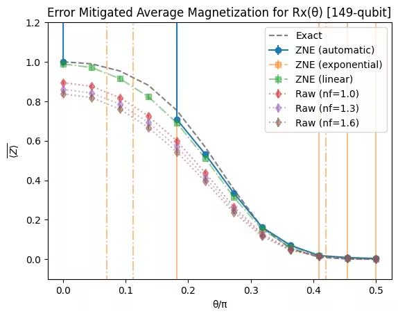
Habang ang mga maingay na halaga (noise factor nf=1.0) ay nagpapakita ng malaking paglihis mula sa mga eksaktong halaga, ang mga mitigated na halaga ay malapit sa mga eksaktong halaga, na nagpapatunay ng pagiging kapaki-pakinabang ng PEA-based mitigation technique.
I-plot ang mga resulta ng extrapolation para sa mga indibidwal na qubit
Sa wakas, ang sumusunod na code ay gumagawa ng plot upang ipakita ang mga extrapolation curve para sa iba't ibang halaga ng theta sa isang partikular na qubit.
zne_metadata = primitive_result.metadata["resilience"]["zne"]
# Plot Trotter simulation results
fig = plot_trotter_results(
    pub_result,
    parameter_values,
    plot_extrapolator=zne_metadata["extrapolator"],
    plot_noise_factors=zne_metadata["noise_factors"],
    exact=exact_data,
)
display(fig)
virtual_qubit = 1
plot_qubit_zne_data(
    pub_result=pub_result,
    angles=parameter_values,
    qubit=virtual_qubit,
    noise_factors=zne_metadata["noise_factors"],
    extrapolator=zne_metadata["extrapolator"],
    extrapolated_noise_factors=zne_metadata["extrapolated_noise_factors"],
)
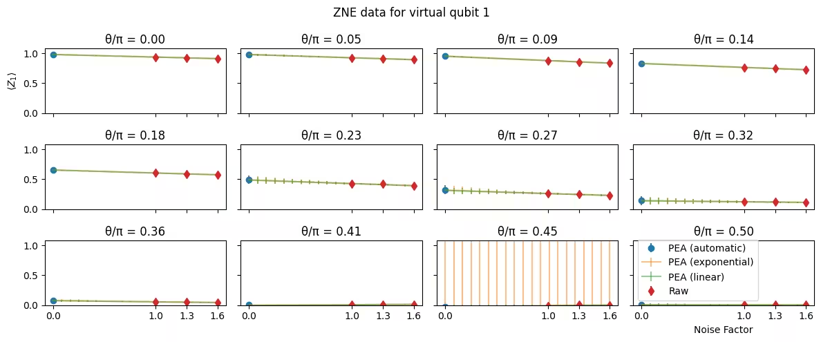
Mga susunod na hakbang
Kung nahanap mong kawili-wili ang gawaing ito, maaaring interesado ka sa mga sumusunod na materyal:
- Isang tutorial na nakatuon sa pagsasama ng mga teknik sa pagbabawas ng error.
- Detalyadong dokumentasyon sa mga teknik sa pagbabawas ng error na available sa Qiskit.
- Mga karagdagang aralin na sumasaklaw sa mga utility-scale na eksperimento: Utility II at Utility III.