Sample-based quantum diagonalization ng isang chemistry Hamiltonian

Tantiya ng paggamit: mas mababa sa isang minuto sa isang Heron r2 processor (PAALALA: Ito ay tantiya lamang. Ang iyong runtime ay maaaring mag-iba.)

Mga resulta ng pag-aaral

Pagkatapos ng tutorial na ito, dapat maunawaan ng mga gumagamit ang:

• Paano gamitin ang SQD Qiskit addon upang tantiyahin ang ground state energy ng isang molecular system gamit ang mga bitstrings na na-sample mula sa isang quantum processing unit (QPU).
• Paano gamitin ang ffsim upang bumuo ng local unitary cluster Jastrow (LUCJ) circuit para sa quantum chemistry simulation.

Mga kinakailangan

Inirerekomenda naming pamilyarisehin ng mga gumagamit ang sumusunod na mga paksa bago gawin ang tutorial na ito:

• Quantum chemistry at second quantization
• Paggamit ng Sampler primitive upang mag-sample mula sa quantum circuits

Background

Sa tutorial na ito, ipapakita natin kung paano mag-post-process ng maingay na quantum samples upang tantiyahin ang ground state ng nitrogen molecule $\text{N}_2$ sa equilibrium bond length, sa pamamagitan ng paggamit ng SQD Qiskit addon upang ipatupad ang sample-based quantum diagonalization (SQD) algorithm. Mas maraming detalye sa software ay matatagpuan sa kaukulang dokumentasyon, kabilang ang isang simple example upang makapagsimula.

Ang tutorial na ito ay inirerekomenda para sa mga gumagamit na pamilyar sa quantum chemistry: partikular, ang pagkilala sa paghahanap ng ground state energies ng isang molekula. Para sa detalyadong walkthrough ng workflow, sumangguni sa quantum diagonalization algorithm course.

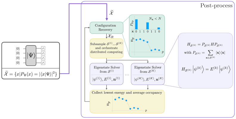
Ang SQD ay isang teknik para sa paghahanap ng eigenvalues at eigenvectors ng quantum operators, tulad ng isang quantum system Hamiltonian, sa pamamagitan ng paggamit ng quantum at distributed classical computing nang magkasama. Ang classical distributed computing ay ginagamit upang mag-proseso ng mga samples na nakuha mula sa isang quantum processor, at upang mag-project at mag-diagonalize ng isang target Hamiltonian sa isang subspace na spanned nito. Ang isang SQD-based workflow ay may sumusunod na hakbang:

1. Pumili ng circuit ansatz at ilapat ito sa isang quantum computer sa isang reference state (sa kasong ito, ang Hartree-Fock state).
2. Mag-sample ng mga bitstrings mula sa resultang quantum state.
3. Patakbuhin ang self-consistent configuration recovery procedure sa mga bitstrings upang makuha ang approximation sa ground state.

Ang SQD ay kilala na gumagana nang maayos kapag ang target eigenstate ay sparse: ang wave function ay sinusuportahan sa isang set ng basis states $\mathcal{S} = \{|x\rangle \}$ na ang laki ay hindi tumataas nang exponentially sa laki ng problema.

Quantum chemistry

Ang Hamiltonian ng isang molecular system ay maaaring isulat bilang

$$\hat{H} = \sum_{ \substack{pr\\\sigma} } h_{pr} \, \hat{a}^\dagger_{p\sigma} \hat{a}_{r\sigma} + \frac12 \sum_{ \substack{prqs\\\sigma\tau} } h_{prqs} \, \hat{a}^\dagger_{p\sigma} \hat{a}^\dagger_{q\tau} \hat{a}_{s\tau} \hat{a}_{r\sigma},$$

kung saan ang $h_{pr}$ at $h_{prqs}$ ay mga complex numbers na tinatawag na molecular integrals na maaaring kalkulahin mula sa specification ng molekula gamit ang isang computer program. Sa tutorial na ito, kinakalkula natin ang mga integrals gamit ang PySCF software package.

Para sa mga detalye tungkol sa kung paano na-derive ang molecular Hamiltonian, kumonsulta sa isang textbook sa quantum chemistry (halimbawa, Modern Quantum Chemistry ni Szabo at Ostlund). Para sa isang high-level explanation kung paano ang quantum chemistry problems ay nima-map sa quantum computers, tingnan ang lecture na Mapping Problems to Qubits mula sa Qiskit Global Summer School 2024.

Local unitary cluster Jastrow (LUCJ) ansatz

Ang SQD ay nangangailangan ng isang quantum circuit ansatz upang kumuha ng mga samples. Sa tutorial na ito, gagamitin natin ang local unitary cluster Jastrow (LUCJ) ansatz dahil sa kombinasyon nito ng physical motivation at hardware-friendliness. Gagamitin natin ang ffsim upang itayo ang ansatz circuit.

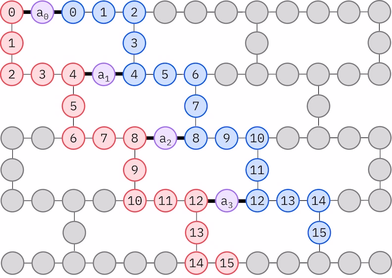
Ang LUCJ ansatz ay nag-aadapt sa mga QPU na may limitadong qubit connectivity. Ang mga spin orbital ay nima-map sa mga qubit upang ang ansatz ay hindi nangangailangan ng routing gamit ang mga SWAP gate. Ang IBM® hardware ay may heavy-hex lattice qubit topology, sa kasong iyon maaari tayong gumamit ng "zig-zag" pattern, na inilalarawan sa ibaba. Sa pattern na ito, ang mga orbitals na may parehong spin ay nima-map sa mga qubits na may line topology (pula at asul na bilog), at ang koneksyon sa pagitan ng mga orbitals na may ibang spin ay naroroon sa bawat ika-4 na spatial orbital, na ang koneksyon ay pinadadali ng isang ancilla qubit (lila na bilog).

Self-consistent configuration recovery

Ang self-consistent configuration recovery procedure ay dinisenyo upang kunin ang pinakamaraming signal hangga't maaari mula sa maingay na quantum samples. Dahil ang molecular Hamiltonian ay nag-conserve ng particle number at spin Z, may katuturan na pumili ng circuit ansatz na nag-conserve din ng mga symmetrya na ito. Kapag inilapat sa Hartree-Fock state, ang resultang state ay may fixed particle number at spin Z sa noiseless setting. Samakatuwid, ang spin-$\alpha$ at spin-$\beta$ halves ng anumang bitstring na na-sample mula sa state na ito ay dapat magkaroon ng parehong Hamming weight tulad ng sa Hartree-Fock state. Dahil sa presensya ng noise sa kasalukuyang quantum processors, ang ilang nasukat na bitstrings ay lalabag sa property na ito. Ang isang simpleng anyo ng postselection ay magtatapon ng mga bitstrings na ito, ngunit sayang ito dahil ang mga bitstrings na iyon ay maaaring maglaman pa ng ilang signal. Ang self-consistent recovery procedure ay sinusubukang mabawi ang ilan sa signal na iyon sa post-processing. Ang procedure ay iterative at nangangailangan bilang input ng isang tantiya ng average occupancies ng bawat orbital sa ground state, na unang kinakalkula mula sa raw samples. Ang procedure ay pinapatakbo sa isang loop, at bawat iteration ay may sumusunod na mga hakbang:

1. Para sa bawat bitstring na lumalabag sa tinukoy na mga symmetrya, i-flip ang mga bits nito gamit ang isang probabilistic procedure na dinisenyo upang dalhin ang bitstring nang mas malapit sa kasalukuyang tantiya ng average orbital occupancies, upang makakuha ng bagong bitstring.
2. Kolektahin ang lahat ng lumang at bagong bitstrings na nakakatugon sa mga symmetrya, at mag-subsample ng mga subsets ng fixed size, na pinili nang maaga.
3. Para sa bawat subset ng bitstrings, i-project ang Hamiltonian sa subspace na spanned ng kaukulang basis vectors (tingnan ang nakaraang seksyon para sa paglalarawan ng mga basis vectors na ito), at kalkulahin ang ground state estimate ng projected Hamiltonian sa isang classical computer.
4. I-update ang tantiya ng average orbital occupancies gamit ang ground state estimate na may pinakamababang energy.

SQD workflow diagram

Ang SQD workflow ay inilalarawan sa sumusunod na diagram:

Requirements

Bago simulan ang tutorial na ito, tiyaking mayroon kang sumusunod na naka-install:

• Qiskit SDK v1.0 o mas bago, na may visualization support
• Qiskit Runtime v0.22 o mas bago (pip install qiskit-ibm-runtime)
• SQD Qiskit addon v0.11 o mas bago (pip install qiskit-addon-sqd)
• ffsim v0.0.75 o mas bago (pip install ffsim)

Setup

# Added by doQumentation — required packages for this notebook
!pip install -q ffsim matplotlib numpy pyscf qiskit qiskit-addon-sqd qiskit-ibm-runtime

import math

import ffsim
import matplotlib.pyplot as plt
import numpy as np
import pyscf
import pyscf.cc
import pyscf.mcscf
from qiskit import QuantumCircuit, QuantumRegister
from qiskit.primitives import StatevectorSampler
from qiskit.providers.fake_provider import GenericBackendV2
from qiskit_ibm_runtime import QiskitRuntimeService
from qiskit_ibm_runtime import SamplerV2 as Sampler

Maliit na halimbawa ng simulator

Sa tutorial na ito, hahanapin natin ang approximation sa ground state ng nitrogen molecule malapit sa equilibrium bond distance nito. Gagamitin muna natin ang isang maliit na STO-6G basis set upang masimulate natin ang eksperimento at masiguro na gumagana ito.

Hakbang 1: I-map ang mga classical inputs sa isang quantum problem

Una, tutukuyin natin ang molekula at ang mga katangian nito.

# Specify molecule properties
spin_sq = 0

# Build N2 molecule
mol = pyscf.gto.Mole()
mol.build(
    atom=[["N", (0, 0, 0)], ["N", (1.0, 0, 0)]],
    basis="sto-6g",
    symmetry="Dooh",
)

# Define active space
n_frozen = 2
active_space = range(n_frozen, mol.nao_nr())

# Get molecular integrals
scf = pyscf.scf.RHF(mol).run()
norb = len(active_space)
n_electrons = int(sum(scf.mo_occ[active_space]))
n_alpha = (n_electrons + mol.spin) // 2
n_beta = (n_electrons - mol.spin) // 2
nelec = (n_alpha, n_beta)
cas = pyscf.mcscf.CASCI(scf, norb, nelec)
mo = cas.sort_mo(active_space, base=0)
hcore, nuclear_repulsion_energy = cas.get_h1cas(mo)
eri = pyscf.ao2mo.restore(1, cas.get_h2cas(mo), norb)

# Compute exact energy using FCI
reference_energy = cas.run().e_tot

print(f"norb = {norb}")
print(f"nelec = {nelec}")

converged SCF energy = -108.464957764796
CASCI E = -108.595987350986  E(CI) = -32.4115475088426  S^2 = 0.0000000
norb = 8
nelec = (5, 5)

Bago itayo ang LUCJ ansatz circuit, magsasagawa muna tayo ng CCSD calculation sa sumusunod na code cell. Ang $t_1$ at $t_2$ amplitudes mula sa calculation na ito ay gagamitin upang i-initialize ang mga parameters ng ansatz.

# Get CCSD t2 amplitudes for initializing the ansatz
ccsd = pyscf.cc.CCSD(
    scf, frozen=[i for i in range(mol.nao_nr()) if i not in active_space]
).run()
t1 = ccsd.t1
t2 = ccsd.t2

E(CCSD) = -108.5933309085008  E_corr = -0.1283731437052354

Ngayon, gagamitin natin ang ffsim upang likhain ang ansatz circuit. Dahil ang ating molekula ay may closed-shell Hartree-Fock state, gagamitin natin ang spin-balanced variant ng UCJ ansatz, UCJOpSpinBalanced. Itatakda natin ang optimize=True sa from_t_amplitudes method upang paganahin ang "compressed" double-factorization ng $t_2$ amplitudes (tingnan ang The local unitary cluster Jastrow (LUCJ) ansatz sa documentation ng ffsim para sa mga detalye).

Dahil ang LUCJ ansatz ay nag-aadapt sa available connectivity ng QPU, kailangan nating i-initialize ang QPU backend bago likhain ang ansatz. Sa ngayon, lilikha tayo ng generic backend na may heavy-hex coupling map at gate set na natural na na-decompose ang LUCJ ansatz. Pagkatapos, gagamitin natin ang ffsim.qiskit.generate_lucj_pass_manager upang lumikha ng pass manager na espesyalista sa pag-transpile ng LUCJ ansatz sa ibinigay na backend ayon sa "zig-zag" layout na inilarawan sa background section sa LUCJ ansatz. Ang function na ito ay gumagamit ng scoring heuristic upang mabawasan ang mga errors na nauugnay sa napiling layout, na mahalaga kung ang iyong backend ay isang tunay na QPU, o isang simulator na may noise model. Bukod sa pagbabalik ng pass manager, nagbabalik din ang function na ito ng alpha-beta coupling pairs na maaaring ipatupad sa hardware. Kung hindi lahat ng pairs ay maaaring ipatupad, maglalabas ito ng babala.

import warnings

from qiskit.transpiler import CouplingMap

warnings.formatwarning = lambda msg, *args, **kwargs: f"Warning: {msg}\n"

# Set ansatz properties
n_reps = 1
pairs_aa = [(p, p + 1) for p in range(norb - 1)]
pairs_ab = None  # Let generate_lucj_pass_manager determine the alpha-beta interactions

# Initialize backend
coupling_map = CouplingMap.from_heavy_hex(3)
backend = GenericBackendV2(
    coupling_map.size(),
    coupling_map=coupling_map,
    basis_gates=["cp", "xx_plus_yy", "p", "x", "swap"],
)

# Create pass manager
pass_manager, pairs_ab = ffsim.qiskit.generate_lucj_pass_manager(
    backend=backend,
    norb=norb,
    connectivity="heavy-hex",
    interaction_pairs=(pairs_aa, pairs_ab),
    optimization_level=3,
)

# Create the LUCJ ansatz operator
ucj_op = ffsim.UCJOpSpinBalanced.from_t_amplitudes(
    t2=t2,
    t1=t1,
    n_reps=n_reps,
    interaction_pairs=(pairs_aa, pairs_ab),
    # Setting optimize=True enables the "compressed" factorization
    optimize=True,
    # Limit the number of optimization iterations to prevent the code cell from running
    # too long. Removing this line may improve results.
    options=dict(maxiter=1000),
)

# create an empty quantum circuit
qubits = QuantumRegister(2 * norb, name="q")
circuit = QuantumCircuit(qubits)

# prepare Hartree-Fock state as the reference state and append it to the quantum circuit
circuit.append(ffsim.qiskit.PrepareHartreeFockJW(norb, nelec), qubits)

# apply the UCJ operator to the reference state
circuit.append(ffsim.qiskit.UCJOpSpinBalancedJW(ucj_op), qubits)
circuit.measure_all()

Hakbang 2: I-optimize para sa quantum hardware execution

Susunod, io-optimize natin ang circuit para sa isang target hardware. Karaniwang kasama sa hakbang na ito ang pag-initialize ng hardware backend at isang pass manager para sa backend na iyon. Gayunpaman, dahil ang LUCJ ansatz ay nag-aadapt sa hardware connectivity, ginawa na natin ang mga aksyon na ito sa nakaraang hakbang. Ang natitira na lang ay patakbuhin ang pass manager sa circuit upang ma-transpile ito sa isang ISA circuit na maaaring direktang i-execute sa QPU.

isa_circuit = pass_manager.run(circuit)
print(f"Gate counts: {isa_circuit.count_ops()}")

Gate counts: OrderedDict({'xx_plus_yy': 86, 'p': 16, 'measure': 16, 'cp': 15, 'x': 10, 'swap': 2, 'barrier': 1})

Hakbang 3: I-execute gamit ang Qiskit primitives

Pagkatapos i-optimize ang circuit para sa hardware execution, handa na tayong patakbuhin ito sa target hardware at mangolekta ng samples para sa ground state energy estimation. Dahil mayroon lamang tayong isang circuit, gagamitin natin ang Qiskit Runtime's Job execution mode at i-execute ang ating circuit.

rng = np.random.default_rng()
sampler = StatevectorSampler(seed=rng)
job = sampler.run([isa_circuit], shots=100_000)

Warning: Trying to add QuantumRegister to a QuantumCircuit having a layout

primitive_result = job.result()
pub_result = primitive_result[0]

Hakbang 4: Mag-post-process at ibalik ang resulta sa gustong classical format

Ang isang kapaki-pakinabang na sukatan upang husgahan ang kalidad ng output ng QPU ay ang bilang ng mga valid na configuration na ibinalik. Ang isang valid na configuration ay may tamang particle number at spin Z, na nangangahulugang ang kanang kalahati ng bitstring ay may Hamming weight na katumbas ng bilang ng spin-up electrons, at ang kaliwang kalahati ay may Hamming weight na katumbas ng bilang ng spin-down electrons. Ang sumusunod na cell ay kinakalkula ang fraction ng mga na-sample na configuration na valid.

def is_valid_bitstring(
    bitstring: str, norb: int, nelec: tuple[int, int]
) -> bool:
    n_alpha, n_beta = nelec
    return (
        len(bitstring) == 2 * norb
        and bitstring[norb:].count("1") == n_alpha
        and bitstring[:norb].count("1") == n_beta
    )

bit_array = pub_result.data.meas
num_valid = sum(
    is_valid_bitstring(b, norb, nelec) for b in bit_array.get_bitstrings()
)
valid_fraction = num_valid / bit_array.num_shots
print(f"Fraction of sampled configurations that are valid: {valid_fraction}")

Fraction of sampled configurations that are valid: 1.0

All of the bitstrings are valid because we are sampling the circuit on a noiseless simulator. When running on a noisy QPU, the fraction will be less than one, but hopefully it will be larger than the fraction you would expect if the bitstrings were sampled uniformly at random, which is computed in the following cell.

expected_fraction_random = (
    math.comb(norb, n_alpha) * math.comb(norb, n_beta) / 2 ** (2 * norb)
)
print(
    f"Expected fraction of valid configurations from uniformly random bitstrings: {expected_fraction_random}"
)

Expected fraction of valid configurations from uniformly random bitstrings: 0.0478515625

Ngayon, tatantiyahin natin ang ground state energy ng Hamiltonian gamit ang diagonalize_fermionic_hamiltonian function. Ginagawa ng function na ito ang self-consistent configuration recovery procedure upang iteratively pag-refine ang maingay na quantum samples upang mapabuti ang energy estimate. Ipapasa natin ang isang callback function upang mai-save natin ang intermediate results para sa paglaon na pagsusuri. Tingnan ang API documentation para sa mga paliwanag ng mga arguments sa diagonalize_fermionic_hamiltonian.

from functools import partial

from qiskit_addon_sqd.fermion import (
    SCIResult,
    diagonalize_fermionic_hamiltonian,
    solve_sci_batch,
)

# SQD options
energy_tol = 1e-3
occupancies_tol = 1e-3
max_iterations = 5

# Eigenstate solver options
num_batches = 3
samples_per_batch = 300
symmetrize_spin = True
carryover_threshold = 1e-4
max_cycle = 200

# Use the Hartree-Fock configuration as an initial guess for the orbital occupancies
initial_occupancies = (
    np.array([1] * n_alpha + [0] * (norb - n_alpha)),
    np.array([1] * n_beta + [0] * (norb - n_beta)),
)

# Pass options to the built-in eigensolver. If you just want to use the defaults,
# you can omit this step, in which case you would not specify the sci_solver argument
# in the call to diagonalize_fermionic_hamiltonian below.
sci_solver = partial(solve_sci_batch, spin_sq=0.0, max_cycle=max_cycle)

# List to capture intermediate results
result_history = []

def callback(results: list[SCIResult]):
    result_history.append(results)
    iteration = len(result_history)
    print(f"Iteration {iteration}")
    for i, result in enumerate(results):
        print(f"\tSubsample {i}")
        print(f"\t\tEnergy: {result.energy + nuclear_repulsion_energy}")
        print(
            f"\t\tSubspace dimension: {np.prod(result.sci_state.amplitudes.shape)}"
        )

result = diagonalize_fermionic_hamiltonian(
    hcore,
    eri,
    bit_array,
    samples_per_batch=samples_per_batch,
    norb=norb,
    nelec=nelec,
    num_batches=num_batches,
    energy_tol=energy_tol,
    occupancies_tol=occupancies_tol,
    max_iterations=max_iterations,
    sci_solver=sci_solver,
    symmetrize_spin=symmetrize_spin,
    initial_occupancies=initial_occupancies,
    carryover_threshold=carryover_threshold,
    callback=callback,
    seed=rng,
)

final_energy = result.energy + nuclear_repulsion_energy
energy_error = final_energy - reference_energy
print(f"Final energy: {final_energy}")
print(f"Final energy error: {energy_error}")

Iteration 1
	Subsample 0
		Energy: -108.59275573641656
		Subspace dimension: 900
	Subsample 1
		Energy: -108.59275573641656
		Subspace dimension: 900
	Subsample 2
		Energy: -108.59275573641656
		Subspace dimension: 900
Iteration 2
	Subsample 0
		Energy: -108.59275573641656
		Subspace dimension: 900
	Subsample 1
		Energy: -108.59275573641656
		Subspace dimension: 900
	Subsample 2
		Energy: -108.59275573641656
		Subspace dimension: 900
Final energy: -108.59275573641656
Final energy error: 0.0032316145694579745

Mga resulta ng biswal

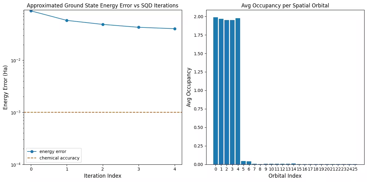
Ang unang plot ay nagpapakita na sa simulation na ito ay nasa loob na tayo ng 1 mH ng tamang sagot pagkatapos ng unang iteration (ang chemical accuracy ay karaniwang tinatanggap na 1 kcal/mol $\approx$ 1.6 mH). Ito ay isang maliit na sistema, at dahil ang mga samples ay walang ingay, hindi kailangan ng configuration recovery. Sa isang mas malaking sistema na pinatakbo sa isang maingay na QPU, maaaring kailanganin ang maraming configuration recovery iterations, at ang panghuling katumpakan ay maaaring mas masama. Sa pangkalahatan, ang energy ay maaaring mapabuti sa pamamagitan ng pagpapahintulot ng mas maraming configuration recovery iterations o sa pamamagitan ng pagtaas ng bilang ng samples per batch.

Ang pangalawang plot ay nagpapakita ng average occupancy ng bawat spatial orbital pagkatapos ng huling iteration. Makikita natin na parehong ang spin-up at spin-down electrons ay nag-occupy ng unang limang orbitals na may mataas na probability sa ating mga solusyon.

# Data for energies plot
x1 = range(len(result_history))
min_e = [
    min(result, key=lambda res: res.energy).energy + nuclear_repulsion_energy
    for result in result_history
]
e_diff = [abs(e - reference_energy) for e in min_e]
yt1 = [1.0, 1e-1, 1e-2, 1e-3, 1e-4]

# Chemical accuracy (+/- 1 milli-Hartree)
chem_accuracy = 0.001

# Data for avg spatial orbital occupancy
y2 = np.sum(result.orbital_occupancies, axis=0)
x2 = range(len(y2))

fig, axs = plt.subplots(1, 2, figsize=(12, 6))

# Plot energies
axs[0].plot(x1, e_diff, label="energy error", marker="o")
axs[0].set_xticks(x1)
axs[0].set_xticklabels(x1)
axs[0].set_yticks(yt1)
axs[0].set_yticklabels(yt1)
axs[0].set_yscale("log")
axs[0].set_ylim(1e-4)
axs[0].axhline(
    y=chem_accuracy,
    color="#BF5700",
    linestyle="--",
    label="chemical accuracy",
)
axs[0].set_title("Approximated Ground State Energy Error vs SQD Iterations")
axs[0].set_xlabel("Iteration Index", fontdict={"fontsize": 12})
axs[0].set_ylabel("Energy Error (Ha)", fontdict={"fontsize": 12})
axs[0].legend()

# Plot orbital occupancy
axs[1].bar(x2, y2, width=0.8)
axs[1].set_xticks(x2)
axs[1].set_xticklabels(x2)
axs[1].set_title("Avg Occupancy per Spatial Orbital")
axs[1].set_xlabel("Orbital Index", fontdict={"fontsize": 12})
axs[1].set_ylabel("Avg Occupancy", fontdict={"fontsize": 12})

plt.tight_layout()
plt.show()

Halimbawa ng malaking sukat sa tunay na hardware

Ngayon, magpapatakbo tayo ng mas malaking halimbawa sa tunay na quantum hardware. Dito, magdaderi tayo ng active space para sa nitrogen molecule mula sa cc-pVDZ basis set.

Mga Hakbang 1-4

Dito pinagsasama natin ang lahat ng hakbang sa isang solong workflow sa mas malaking sukat, na pagkatapos ay pinapatakbo sa tunay na quantum hardware.

# ------------------------------ Step 1 ------------------------------
# Build N2 molecule
mol = pyscf.gto.Mole()
mol.build(
    atom=[["N", (0, 0, 0)], ["N", (1.0, 0, 0)]],
    basis="cc-pvdz",
    symmetry="Dooh",
)

# Define active space
n_frozen = 2
active_space = range(n_frozen, mol.nao_nr())

# Get molecular integrals
scf = pyscf.scf.RHF(mol).run()
norb = len(active_space)
n_electrons = int(sum(scf.mo_occ[active_space]))
n_alpha = (n_electrons + mol.spin) // 2
n_beta = (n_electrons - mol.spin) // 2
nelec = (n_alpha, n_beta)
cas = pyscf.mcscf.CASCI(scf, norb, nelec)
mo = cas.sort_mo(active_space, base=0)
hcore, nuclear_repulsion_energy = cas.get_h1cas(mo)
eri = pyscf.ao2mo.restore(1, cas.get_h2cas(mo), norb)

# Store reference energy from SCI calculation performed separately
reference_energy = -109.22802921665716

print(f"norb = {norb}")
print(f"nelec = {nelec}")

# Get CCSD t2 amplitudes for initializing the ansatz
ccsd = pyscf.cc.CCSD(
    scf, frozen=[i for i in range(mol.nao_nr()) if i not in active_space]
).run()
t1 = ccsd.t1
t2 = ccsd.t2

# Set ansatz properties
n_reps = 1
pairs_aa = [(p, p + 1) for p in range(norb - 1)]
pairs_ab = None  # Let generate_lucj_pass_manager determine the alpha-beta interactions

# Initialize backend
service = QiskitRuntimeService()
backend = service.least_busy(
    operational=True, simulator=False, min_num_qubits=133
)
print(f"Using backend {backend.name}")

# Create pass manager
pass_manager, pairs_ab = ffsim.qiskit.generate_lucj_pass_manager(
    backend=backend,
    norb=norb,
    connectivity="heavy-hex",
    interaction_pairs=(pairs_aa, pairs_ab),
    optimization_level=3,
)

# Create the LUCJ ansatz operator
ucj_op = ffsim.UCJOpSpinBalanced.from_t_amplitudes(
    t2=t2,
    t1=t1,
    n_reps=n_reps,
    interaction_pairs=(pairs_aa, pairs_ab),
    # Setting optimize=True enables the "compressed" factorization
    optimize=True,
    # Limit the number of optimization iterations to prevent the code cell from running
    # too long. Removing this line may improve results.
    options=dict(maxiter=1000),
)

# create an empty quantum circuit
qubits = QuantumRegister(2 * norb, name="q")
circuit = QuantumCircuit(qubits)

# prepare Hartree-Fock state as the reference state and append it to the quantum circuit
circuit.append(ffsim.qiskit.PrepareHartreeFockJW(norb, nelec), qubits)

# apply the UCJ operator to the reference state
circuit.append(ffsim.qiskit.UCJOpSpinBalancedJW(ucj_op), qubits)
circuit.measure_all()

# ------------------------------ Step 2 ------------------------------

isa_circuit = pass_manager.run(circuit)
print(f"Gate counts: {isa_circuit.count_ops()}")

# ------------------------------ Step 3 ------------------------------
sampler = Sampler(mode=backend)
sampler.options.environment.job_tags = ["TUT_SQD"]
job = sampler.run([isa_circuit], shots=100_000)
primitive_result = job.result()
pub_result = primitive_result[0]

# ------------------------------ Step 4 ------------------------------

bit_array = pub_result.data.meas
num_valid = sum(
    is_valid_bitstring(b, norb, nelec) for b in bit_array.get_bitstrings()
)
valid_fraction = num_valid / bit_array.num_shots
print(f"Fraction of sampled configurations that are valid: {valid_fraction}")
expected_fraction_random = (
    math.comb(norb, n_alpha) * math.comb(norb, n_beta) / 2 ** (2 * norb)
)
print(
    f"Expected fraction of valid configurations from uniformly random bitstrings: {expected_fraction_random}"
)
# SQD options
energy_tol = 1e-3
occupancies_tol = 1e-3
max_iterations = 5

# Eigenstate solver options
num_batches = 3
samples_per_batch = 300
symmetrize_spin = True
carryover_threshold = 1e-4
max_cycle = 200

# Use the Hartree-Fock configuration as an initial guess for the orbital occupancies
initial_occupancies = (
    np.array([1] * n_alpha + [0] * (norb - n_alpha)),
    np.array([1] * n_beta + [0] * (norb - n_beta)),
)

# Pass options to the built-in eigensolver. If you just want to use the defaults,
# you can omit this step, in which case you would not specify the sci_solver argument
# in the call to diagonalize_fermionic_hamiltonian below.
sci_solver = partial(solve_sci_batch, spin_sq=0.0, max_cycle=max_cycle)

# List to capture intermediate results
result_history = []

result = diagonalize_fermionic_hamiltonian(
    hcore,
    eri,
    bit_array,
    samples_per_batch=samples_per_batch,
    norb=norb,
    nelec=nelec,
    num_batches=num_batches,
    energy_tol=energy_tol,
    occupancies_tol=occupancies_tol,
    max_iterations=max_iterations,
    sci_solver=sci_solver,
    symmetrize_spin=symmetrize_spin,
    initial_occupancies=initial_occupancies,
    carryover_threshold=carryover_threshold,
    callback=callback,
    seed=rng,
)

final_energy = result.energy + nuclear_repulsion_energy
energy_error = final_energy - reference_energy
print(f"Final energy: {final_energy}")
print(f"Final energy error: {energy_error}")

# Data for energies plot
x1 = range(len(result_history))
min_e = [
    min(result, key=lambda res: res.energy).energy + nuclear_repulsion_energy
    for result in result_history
]
e_diff = [abs(e - reference_energy) for e in min_e]
yt1 = [1.0, 1e-1, 1e-2, 1e-3, 1e-4]

# Chemical accuracy (+/- 1 milli-Hartree)
chem_accuracy = 0.001

# Data for avg spatial orbital occupancy
y2 = np.sum(result.orbital_occupancies, axis=0)
x2 = range(len(y2))

fig, axs = plt.subplots(1, 2, figsize=(12, 6))

# Plot energies
axs[0].plot(x1, e_diff, label="energy error", marker="o")
axs[0].set_xticks(x1)
axs[0].set_xticklabels(x1)
axs[0].set_yticks(yt1)
axs[0].set_yticklabels(yt1)
axs[0].set_yscale("log")
axs[0].set_ylim(1e-4)
axs[0].axhline(
    y=chem_accuracy,
    color="#BF5700",
    linestyle="--",
    label="chemical accuracy",
)
axs[0].set_title("Approximated Ground State Energy Error vs SQD Iterations")
axs[0].set_xlabel("Iteration Index", fontdict={"fontsize": 12})
axs[0].set_ylabel("Energy Error (Ha)", fontdict={"fontsize": 12})
axs[0].legend()

# Plot orbital occupancy
axs[1].bar(x2, y2, width=0.8)
axs[1].set_xticks(x2)
axs[1].set_xticklabels(x2)
axs[1].set_title("Avg Occupancy per Spatial Orbital")
axs[1].set_xlabel("Orbital Index", fontdict={"fontsize": 12})
axs[1].set_ylabel("Avg Occupancy", fontdict={"fontsize": 12})

plt.tight_layout()
plt.show()

converged SCF energy = -108.929838385609
norb = 26
nelec = (5, 5)
E(CCSD) = -109.2177884185544  E_corr = -0.2879500329450045
Using backend ibm_boston

Warning: Backend cannot accommodate pairs_ab=[(0, 0), (4, 4), (8, 8), (12, 12), (16, 16), (20, 20), (24, 24)].
Removing interaction (24, 24) from the end.
Warning: Backend cannot accommodate pairs_ab=[(0, 0), (4, 4), (8, 8), (12, 12), (16, 16), (20, 20)].
Removing interaction (20, 20) from the end.

Gate counts: OrderedDict({'sx': 7039, 'rz': 6990, 'cz': 1858, 'x': 61, 'measure': 52, 'barrier': 1})
Fraction of sampled configurations that are valid: 0.02124
Expected fraction of valid configurations from uniformly random bitstrings: 9.607888706852918e-07
Iteration 1
	Subsample 0
		Energy: -109.13889134249762
		Subspace dimension: 120409
	Subsample 1
		Energy: -109.11785470455858
		Subspace dimension: 110889
	Subsample 2
		Energy: -109.13234360554011
		Subspace dimension: 130321
Iteration 2
	Subsample 0
		Energy: -109.16392179579177
		Subspace dimension: 223729
	Subsample 1
		Energy: -109.16281938332986
		Subspace dimension: 223729
	Subsample 2
		Energy: -109.16955816711932
		Subspace dimension: 233289
Iteration 3
	Subsample 0
		Energy: -109.17905772999075
		Subspace dimension: 324900
	Subsample 1
		Energy: -109.17532445048462
		Subspace dimension: 357604
	Subsample 2
		Energy: -109.1733168689756
		Subspace dimension: 348100
Iteration 4
	Subsample 0
		Energy: -109.18437778820451
		Subspace dimension: 474721
	Subsample 1
		Energy: -109.18450164209159
		Subspace dimension: 476100
	Subsample 2
		Energy: -109.18493571190754
		Subspace dimension: 487204
Iteration 5
	Subsample 0
		Energy: -109.18616522497996
		Subspace dimension: 622521
	Subsample 1
		Energy: -109.18652868888333
		Subspace dimension: 644809
	Subsample 2
		Energy: -109.18753326484406
		Subspace dimension: 585225
Final energy: -109.18753326484406
Final energy error: 0.040495951813099396

Mga susunod na hakbang

Recommendations

Kung nakita mong kawili-wili ang gawaing ito, maaaring interesado ka sa sumusunod na materyal:

• Sample-based Krylov quantum diagonalization of a fermionic lattice model - isang kaugnay na tutorial na gumagamit ng time evolution circuits sa halip na variational ansatz
• Scale SQD chemistry workflows with Dice solver - isang pahina na nagpapakita kung paano gamitin ang mas mahusay na Dice software para sa diagonalization
• SQD addon API documentation - sanggunian para sa diagonalize_fermionic_hamiltonian function
• Chemistry beyond the scale of exact diagonalization on a quantum-centric supercomputer - ang papel na batayan ng tutorial na ito