Repetition codes

Tinatayang paggamit: mas mababa sa 10 segundo sa isang Heron processor (TANDAAN: Ito ay isang tantiya lamang. Maaaring mag-iba ang iyong runtime.)

Mga natutunan

• Paano magpatupad ng bit-flip error correction code gamit ang dynamic circuits

• Paano magsukat ng stabilizers para matukoy ang mga quantum error nang hindi nasisira ang encoded na impormasyon

• Paano suriin ang performance ng quantum error correction sa pamamagitan ng paghahambing ng corrected at uncorrected na mga resulta

Mga paunang kailangan

• Dynamic circuits

• Mga pangunahing kaalaman sa quantum error correction

Background

Upang makapaggamit ng real-time quantum error correction (QEC), kailangan mong magkaroon ng kakayahang dinamikong kontrolin ang quantum program flow sa panahon ng execution upang ang mga quantum gate ay maaaring kondisyunin batay sa mga resulta ng pagsukat. Ang tutorial na ito ay nagpapatakbo ng bit-flip code, na isang napakasimpleng anyo ng QEC. Ipinapakita nito ang isang dynamic quantum circuit na makakaprotekta sa isang encoded qubit mula sa isang bit-flip error, at pagkatapos ay sinusuri ang pagganap ng bit-flip code.

Maaari mong samantalahin ang mga karagdagang ancilla qubit at entanglement upang sukatin ang mga stabilizer na hindi nagbabago ng encoded quantum information, habang nagbibigay pa rin sa iyo ng impormasyon tungkol sa ilang uri ng mga error na maaaring naganap. Ang isang quantum stabilizer code ay nag-encode ng $k$ logical qubit sa $n$ physical qubit. Ang mga stabilizer code ay nakatuon sa pagwawasto ng isang discrete error set na may suporta mula sa Pauli group $\Pi^n$.

Sa tutorial na ito, ipinapakita namin ang bit-flip code gamit ang isang simpleng quantum memory experiment. Ihahanda natin ang encoded qubit sa logical state $|\bar{1}\rangle \equiv |111\rangle$ at pagkatapos ay magpapatupad ng maraming cycle ng idle time (para makapag-ipon ng errors) na sinusundan ng error detection at correction. Pagkatapos ay susukatin natin ang probability ng logical error bilang function ng bilang ng cycles (oras), kung saan ang logical error probability ay ang probability na makita ang mga qubit sa isang state na hindi na-recover ang $|\bar{1}\rangle$ pagkatapos ng huling measurement (partikular, ang mga state na katumbas ng error ay $|000\rangle$, $|001\rangle$, $|010\rangle$, at $|100\rangle$).

Ikukumpara natin ang error rate laban sa oras sa mga error rate ng indibidwal, unencoded na mga qubit, at gagamitin rin natin ang repetition code kung saan tinutukoy at itinatama lang natin ang mga error pagkatapos ng huling measurement, ngunit hindi dynamic sa panahon ng circuit.

Tandaan: ang repetition code ay pumapayag lang sa correction ng bit-flip errors kaya hindi ito kumpletong error correction code. Gayunpaman, dahil sa pagiging simple nito, ito ay isang magandang panimulang punto para ipakita kung paano magpatupad ng error correction sa isang quantum computer. Ang memory experiment sa ibaba ay sumusubok lang ng isang uri ng error (isang $|\bar{1}\rangle$ na bumababa sa $|\bar{0}\rangle$) at teknikal na ipinapakita lang nito ang proteksyon ng classical na impormasyon.

Requirements

Bago magsimula sa tutorial na ito, siguraduhing mayroon kang mga sumusunod na naka-install:

• Qiskit SDK v2.0 o mas bago, na may suportang visualization

• Qiskit Runtime v0.40 o mas bago (pip install qiskit-ibm-runtime)

Setup

# Added by doQumentation — installs the packages this notebook needs if they are missing
import importlib.util

_needed = {"matplotlib": "matplotlib", "numpy": "numpy", "qiskit": "qiskit", "qiskit_ibm_runtime": "qiskit-ibm-runtime", "scipy": "scipy", "seaborn": "seaborn"}
_missing = [pip for module, pip in _needed.items()
            if importlib.util.find_spec(module) is None]
# One at a time, so a package that fails to install does not block the others
for _pip in _missing:
    %pip install -q {_pip}
if not _missing:
    print("\u2713 All required packages are installed")

import numpy as np
import seaborn as sns
import matplotlib.pyplot as plt
from scipy.optimize import curve_fit

sns.set()
plt.rc("xtick", labelsize=20)
plt.rc("ytick", labelsize=20)
plt.rc("lines", linewidth=3)
plt.rc("font", size=20)
plt.rc("legend", fontsize="large")
plt.rc("axes", labelsize=20)
plt.rcParams["figure.figsize"] = 15, 6
plt.rcParams["legend.title_fontsize"] = 25

# Qiskit imports
from qiskit import (
    QuantumCircuit,
    QuantumRegister,
    ClassicalRegister,
)

# qiskit-ibm-runtime
from qiskit_ibm_runtime import QiskitRuntimeService, SamplerV2 as Sampler
from qiskit_ibm_runtime.circuit import MidCircuitMeasure

service = QiskitRuntimeService()

Halimbawa ng small-scale simulator

Lalaktawan natin ang hakbang na ito dahil ang layunin ng eksperimentong ito ay sukatin ang lifetime ng logical qubit sa ilalim ng aktwal na hardware noise, tulad ng amplitude damping sa panahon ng idle delays; ang isang noiseless na simulator ay hindi magpapakita ng anumang error na madedetect at maitatama.

Halimbawa ng large-scale hardware

Step 1. Map classical inputs to a quantum problem

Pumili ng backend

Para matukoy ang mga error sa panahon ng circuit, kailangan nating pumili ng backend na may access sa MidCircuitMeasure method (tingnan ang dokumentasyon).

# You can see all backends that support mid-circuit measurements by running the following code.
service.backends(filters=lambda b: "measure_2" in b.supported_instructions)

[<IBMBackend('ibm_pittsburgh')>,
 <IBMBackend('ibm_boston')>,
 <IBMBackend('ibm_kingston')>]

# Choose the least busy backend that supports mid-circuit measurements (`measure_2`).

backend = service.least_busy(
    filters=lambda b: "measure_2" in b.supported_instructions,
    operational=True,
    simulator=False,
    dynamic_circuits=True,
)
# backend = service.backend(backend_name) # alternatively, you could choose a specific backend
print(backend.name)

ibm_boston

Bumuo ng sequence ng bit-flip stabilizer circuits na nagpapatupad ng maraming round ng error detection at correction

Ang bit-flip code ay isa sa pinakasimpleng mga halimbawa ng stabilizer code. Pinoprotektahan nito ang estado laban sa isang bit-flip (X) error sa alinman sa mga encoding qubit. Isaalang-alang ang aksyon ng bit-flip error $X$, na nagmamapa ng $|0\rangle \rightarrow |1\rangle$ at $|1\rangle \rightarrow |0\rangle$ sa alinman sa ating mga qubit, kung gayon mayroon tayong $\epsilon = \{E_0, E_1, E_2 \} = \{IIX, IXI, XII\}$. Ang code ay nangangailangan ng limang qubit: tatlo ang ginagamit upang i-encode ang protektadong estado (ang "data qubits"), at ang natitirang dalawa ay ginagamit bilang mga stabilizer measurement ancilla.

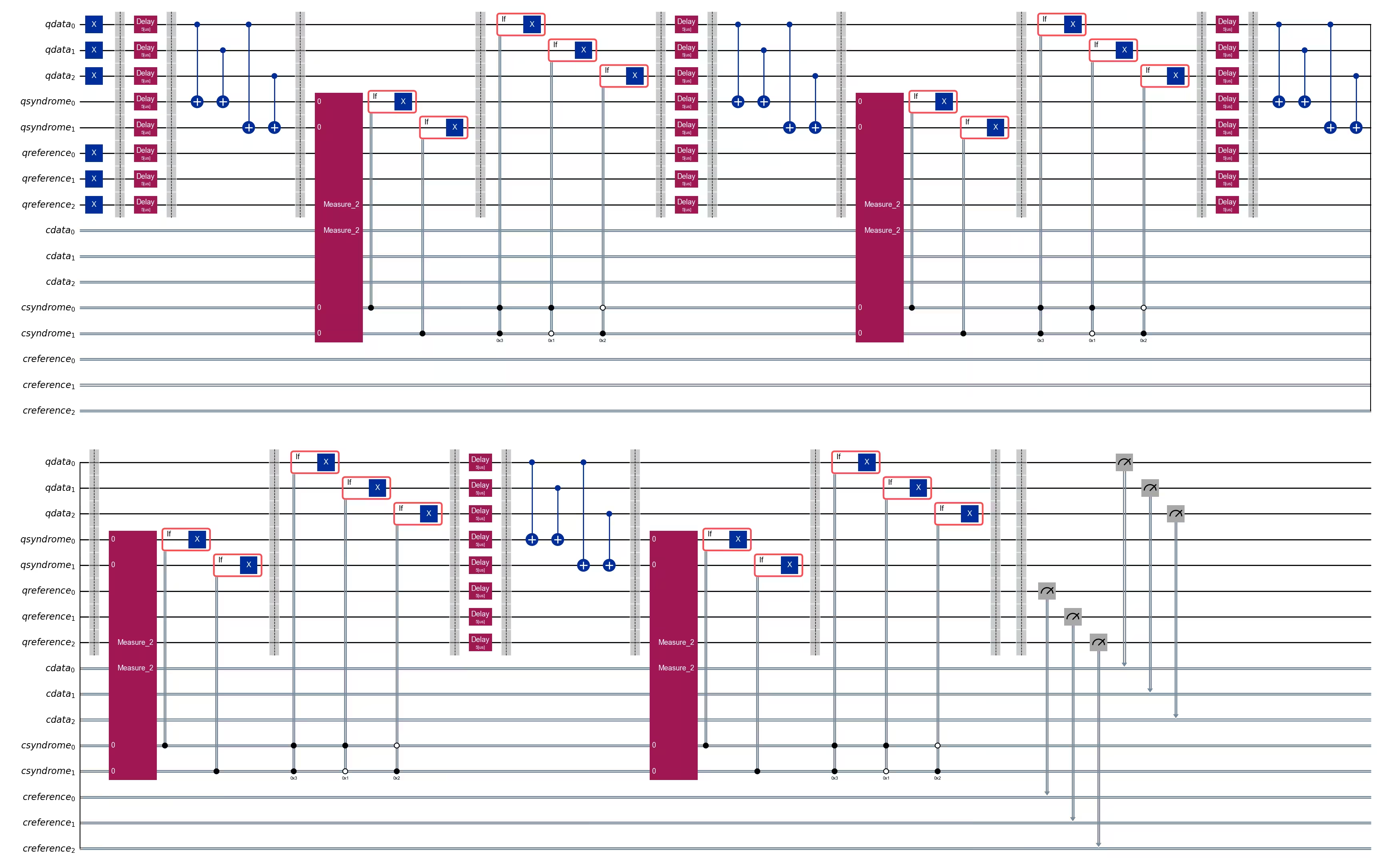
Sa ibaba, bubuo ka ng mga circuit na (1) naghahanda sa data qubits sa logical $|\bar{1} \rangle$ state, pagkatapos ay (2) nagpapatakbo ng maraming cycle ng $5 \mu s$ na delay na sinusundan ng error correction (kasama ang reset ng syndrome qubits), at (3) binabasa ang state ng data qubits.

Susubukan din natin ang lifetime ng $|1\rangle$ state nang hindi gumagamit ng error correction sa pamamagitan ng pagsasama ng tatlong reference qubit na inihahanda natin sa $|1\rangle$ state, iniiwan idle, at pagkatapos ay binabasa.

def build_qc(
    qreg_data,
    qreg_syndrome,
    creg_data,
    creg_syndrome,
    qreg_ref=None,
    creg_ref=None,
):
    """Build a typical error correction circuit"""
    if qreg_ref:
        return QuantumCircuit(
            qreg_data,
            qreg_syndrome,
            creg_data,
            creg_syndrome,
            qreg_ref,
            creg_ref,
        )
    else:
        return QuantumCircuit(
            qreg_data, qreg_syndrome, creg_data, creg_syndrome
        )

def encode_bit_flip(circuit, qreg_data, qreg_ref=None) -> QuantumCircuit:
    """Encode bit-flip. This is done by simply adding a cx"""

    for q in qreg_data:
        circuit.x(q)

    if qreg_ref:
        for q in qreg_ref:
            circuit.x(q)

    circuit.barrier()

    return circuit

def measure_syndrome_bit(
    circuit, qreg_data, qreg_syndrome, creg_syndrome, qreg_ref=None
):
    """
    Measure the syndrome by measuring the parity.
    We reset our ancilla qubits after measuring the stabilizer
    so we can reuse them for repeated stabilizer measurements.
    Because we have already observed the state of the qubit,
    we can write the conditional reset protocol directly to
    avoid another round of qubit measurement if we used
    the `reset` instruction.
    """
    circuit.cx(qreg_data[0], qreg_syndrome[0])
    circuit.cx(qreg_data[1], qreg_syndrome[0])
    circuit.cx(qreg_data[0], qreg_syndrome[1])
    circuit.cx(qreg_data[2], qreg_syndrome[1])
    circuit.barrier()

    for q_measure, c_measure in zip(qreg_syndrome, creg_syndrome):
        circuit.append(MidCircuitMeasure(), [q_measure], [c_measure])

    with circuit.if_test((creg_syndrome[0], 1)):
        circuit.x(qreg_syndrome[0])
    with circuit.if_test((creg_syndrome[1], 1)):
        circuit.x(qreg_syndrome[1])

    circuit.barrier()
    return circuit

def apply_correction_bit(circuit, qreg_data, creg_syndrome):
    """We can detect where an error occurred and correct our state"""
    with circuit.if_test((creg_syndrome, 3)):
        circuit.x(qreg_data[0])
    with circuit.if_test((creg_syndrome, 1)):
        circuit.x(qreg_data[1])
    with circuit.if_test((creg_syndrome, 2)):
        circuit.x(qreg_data[2])
    circuit.barrier()
    return circuit

def apply_final_readout(
    circuit, qreg_data, creg_data, qreg_ref=None, creg_ref=None
):
    """Read out the final measurements"""

    circuit.barrier()
    if qreg_ref:
        circuit.measure(qreg_ref, creg_ref)
    circuit.measure(qreg_data, creg_data)

    return circuit

def build_error_correction_sequence(
    num_cycles, cycles_per_circuit, nq_ref=3, delay=None
) -> QuantumCircuit:
    circuits = []
    reps = []

    qreg_data = QuantumRegister(3, name="qdata")
    qreg_syndrome = QuantumRegister(2, name="qsyndrome")
    creg_data = ClassicalRegister(3, name="cdata")
    creg_syndrome = ClassicalRegister(2, name="csyndrome")
    qreg_ref = QuantumRegister(nq_ref, name="qreference")
    creg_ref = ClassicalRegister(nq_ref, name="creference")

    circuit = build_qc(
        qreg_data,
        qreg_syndrome,
        creg_data,
        creg_syndrome,
        qreg_ref=qreg_ref,
        creg_ref=creg_ref,
    )
    circuit = encode_bit_flip(circuit, qreg_data, qreg_ref=qreg_ref)

    circuit_n = circuit.copy()
    circuit_n = apply_final_readout(
        circuit_n, qreg_data, creg_data, qreg_ref=qreg_ref, creg_ref=creg_ref
    )
    circuits.append(circuit_n)
    reps.append(0)

    for i in range(1, num_cycles + 1):
        if delay:
            circuit.delay(delay, unit="us")
            circuit.barrier()
        circuit = measure_syndrome_bit(
            circuit,
            qreg_data,
            qreg_syndrome,
            creg_syndrome,
            qreg_ref=qreg_ref,
        )
        circuit = apply_correction_bit(circuit, qreg_data, creg_syndrome)
        circuit_n = circuit.copy()
        if i % cycles_per_circuit == 0:
            circuit_n = apply_final_readout(
                circuit_n,
                qreg_data,
                creg_data,
                qreg_ref=qreg_ref,
                creg_ref=creg_ref,
            )
            circuits.append(circuit_n)
            reps.append(i)

    return circuits, np.array(reps)

num_cycles = 40
cycles_per_circuit = 4
nq_ref = 3
circuits, rep_array = build_error_correction_sequence(
    num_cycles, cycles_per_circuit, nq_ref=3, delay=5
)
circuits[1].draw(output="mpl", cregbundle=False, fold=50)

Step 2: I-optimize ang problema para sa pagpapatakbo sa quantum hardware

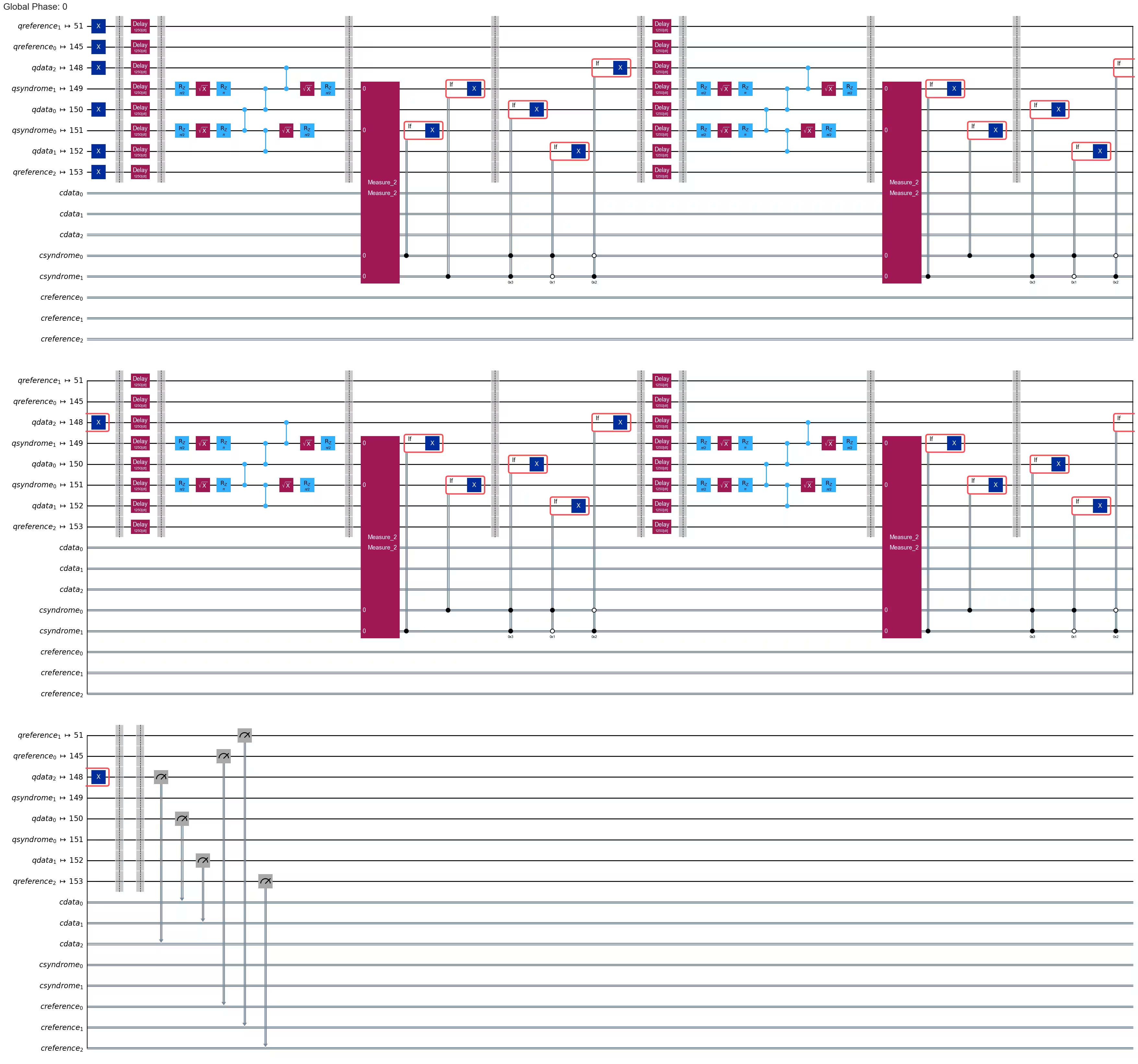
Upang mabawasan ang kabuuang oras ng pagpapatupad ng trabaho, ang mga Qiskit primitive ay tumatanggap lamang ng mga circuit at observable na sumusunod sa mga tagubilin at koneksyon na sinusuportahan ng target system (tinutukoy bilang instruction set architecture (ISA) circuit at observable). Matuto pa tungkol sa transpilation.

Gumawa ng mga ISA circuit

Magsisimula tayo sa paghahanap ng initial layout (ibig sabihin, isang pagpili ng physical qubits kung saan i-map ang ating mga circuit) sa pamamagitan ng pag-transpile ng pinakamahabang circuit natin gamit ang preset pass manager na may optimization level 3.

from qiskit.transpiler.preset_passmanagers import generate_preset_pass_manager

pm = generate_preset_pass_manager(backend=backend, optimization_level=3)
isa_circuit_ref = pm.run(circuits[-1])

init_layout = isa_circuit_ref.layout.initial_index_layout(
    filter_ancillas=True
)
print(init_layout)

[56, 44, 62, 43, 63, 22, 48, 67]

Para sa reference qubits na ikukumpara natin sa ating logical quantum memory, pipiliin natin ang mga ito bilang pinakamahusay na available na qubit sa usapin ng amplitude damping coherence time ($T_1$).

# get all qubits ordered by T1
t1_data = []
for i in range(backend.num_qubits):
    try:
        t1_us = backend.properties().t1(i) * 1e6
    except Exception:
        t1_us = 0.0
    t1_data.append((i, t1_us))

t1_data_sorted = sorted(t1_data, key=lambda x: x[1], reverse=True)

# exclude the qubits we have already mapped the error correcting code to
t1_data_sorted = [
    t1_data for t1_data in t1_data_sorted if t1_data[0] not in init_layout[:5]
]

# use the best qubits in terms of T1 for the reference qubits
init_layout = init_layout[:5] + [t1_data[0] for t1_data in t1_data_sorted[:3]]
print(init_layout)

[56, 44, 62, 43, 63, 143, 131, 31]

# These are the resulting T1 times
properties = backend.properties()
print("Amplitude damping decoherence times for code data qubits:")
for q in init_layout[:3]:
    t1 = properties.t1(q)
    print(f"qubit {q}: T1 = {t1 * 1e6:.0f} mus")

print("\nAmplitude damping decoherence times for reference qubits:")
for q in init_layout[-3:]:
    t1 = properties.t1(q)
    print(f"qubit {q}: T1 = {t1 * 1e6:.0f} mus")

Amplitude damping decoherence times code data qubits:
qubit 56: T1 = 322 mus
qubit 44: T1 = 263 mus
qubit 62: T1 = 290 mus

Amplitude damping decoherence times reference qubits:
qubit 143: T1 = 442 mus
qubit 131: T1 = 410 mus
qubit 31: T1 = 401 mus

# now we transpile all circuits to this initial layout; this way each circuit is run on the same qubits and we can make a fair comparison
pm = generate_preset_pass_manager(
    backend=backend,
    optimization_level=3,
    initial_layout=init_layout,
)
isa_circuits = pm.run(circuits)

isa_circuits[1].draw("mpl", cregbundle=False, fold=50)

Step 3. Execute using Qiskit primitives

sampler = Sampler(mode=backend)

sampler.options.environment.job_tags = ["TUT-REPCODE"]
sampler.options.max_execution_time = 600  # this workload is expected to be under 10s, but it is generally a good habit to set a max execution time (here 600s = 10m)

job = sampler.run(isa_circuits, shots=1000)
print(job.job_id())

job.status()

'DONE'

Step 4: I-post-process at ibalik ang resulta sa nais na classical format

Ikukumpara na natin ngayon ang mga error rate laban sa oras sa pagitan ng logical memory gamit ang 3-qubit repetition code sa isang banda, at ang indibidwal na unencoded na reference qubits sa kabilang banda.

results = job.result()

def correct_counts(counts_dict):
    """
    Corrects the measured logical qubit encoded in the repetition code using majority vote
    """

    result = {"000": 0, "111": 0}
    for bitstring, count in counts_dict.items():
        key = "111" if bitstring.count("1") > 1 else "000"
        result[key] += count
    return result

accuracy = []  # logical qubit
accuracies_ref = np.zeros(
    (len(results), nq_ref)
)  # accuracies on individual reference qubits

for n, pub_result in enumerate(results):
    # logical accuracy (one minus error probability) for active error correction with repetition code
    counts = pub_result.data.cdata.get_counts()
    shots = sum(counts.values())
    counts_corrected = correct_counts(counts)
    accuracy.append(counts_corrected.get("111", 0) / shots)

    # accuracy for individual physical reference qubits without any error correction
    for i in range(nq_ref):
        counts = pub_result.data.creference.slice_bits(i).get_counts()
        accuracies_ref[n, i] = counts.get("1", 0) / shots

accuracy = np.array(accuracy)

def error_proba_t1(N, t1):
    """
    Exponential fitting function for amplitude damping vs. number of cycles
    """

    t_cycle = 7.3e-6  # approximate time per cycle = 5 mus delay + 2.3 mus for error correction
    return 1 - np.exp(-t_cycle * N / t1)

fig, ax = plt.subplots(1, 1, figsize=(15, 5))
ax.plot(
    rep_array, (1.0 - accuracy) * 100.0, "ko-", linewidth=3, label="rep code"
)

for i in range(nq_ref):
    accuracy_1q = accuracies_ref[:, i]
    if i == 0:
        ax.plot(
            rep_array,
            (1.0 - accuracy_1q) * 100.0,
            "go-",
            linewidth=1,
            label="1q reference",
        )
    else:
        ax.plot(rep_array, (1.0 - accuracy_1q) * 100.0, "go-", linewidth=1)

params_bf, pcov = curve_fit(
    error_proba_t1, rep_array, 1.0 - accuracy, bounds=([0, 5e-3])
)
t1_bf = params_bf[0]
print(f"Best-fit effective T1 = {t1_bf * 1e6:.0f} us")
error_prob_bf = error_proba_t1(
    rep_array, t1_bf
)  # np.array([1 - np.exp(-t_cycle * nt/t1) for nt in rep_array])
ax.plot(rep_array, error_prob_bf * 100.0, "k--", linewidth=1)

ax.set_xlabel("error correction rounds")
ax.set_ylabel("error [%]")
ax.set_ylim(bottom=0)
ax.legend(fontsize=15);

Best-fit effective T1 = 1397 us

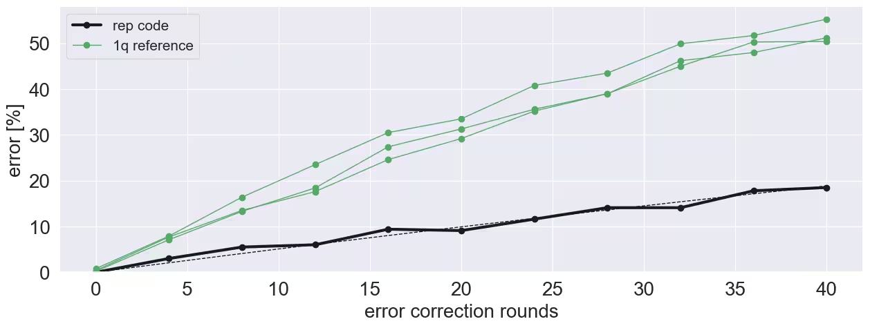
Malinaw nating nakikita ang pinahusay na lifetime ng $|\bar{1}\rangle$ state, kahit ikumpara sa pinakamahusay na (unencoded) physical qubits. Gayunpaman, tandaan na ang eksperimentong ito ay itinatama lang ang isang uri ng error, ibig sabihin ang bit-flips. Kaya mo bang pahusayin ang lifetime ng logical qubit? Maaari mong tuklasin ang pag-optimize ng delay time, pagpapalaki ng sukat ng repetition code lampas sa $n=3$, at iba pa.

Mga susunod na hakbang

Kung interesado ka sa gawaing ito, maaaring maging interesado ka rin sa mga sumusunod na materyal:

Mga Rekomendasyon

• Kurso ng Foundations of quantum error correction - alamin pa ang tungkol sa quantum error correction

• Low-overhead error detection with spacetime codes na tutorial - alamin kung paano gamitin ang Pauli checks para matukoy ang mga error at post-select ang mga sample