Krylov quantum diagonalization ng lattice Hamiltonians

Tantiya sa paggamit: 20 minuto sa Heron r2 (PAALALA: Ito ay tantiya lamang. Maaaring mag-iba ang iyong runtime.)

# Added by doQumentation — required packages for this notebook
!pip install -q matplotlib numpy qiskit qiskit-ibm-runtime scipy sympy

# This cell is hidden from users – it disables some lint rules
# ruff: noqa: E402 E722 F601

Background

Ang tutorial na ito ay nagpapakita kung paano ipatupad ang Krylov Quantum Diagonalization Algorithm (KQD) sa konteksto ng Qiskit patterns. Matututunan mo muna ang teorya sa likod ng algorithm at pagkatapos ay makikita mo ang demonstrasyon ng pagpapatupad nito sa QPU.

Sa iba't ibang disiplina, interesado tayong matutunan ang mga katangian ng ground state ng mga quantum system. Kabilang dito ang pag-unawa sa pundamental na kalikasan ng mga particle at pwersa, paghula at pag-unawa sa pag-uugali ng mga komplikadong materyales, at pag-unawa sa mga bio-chemical na interaksyon at reaksyon. Dahil sa exponential growth ng Hilbert space at sa correlation na lumalabas sa mga entangled system, nahihirapan ang mga classical algorithm na lutasin ang problemang ito para sa mga quantum system na lumalaki ang sukat. Sa isang dulo ng spectrum ay ang umiiral na approach na sumasamantala sa quantum hardware na nakatuon sa mga variational quantum method (halimbawa, variational quantum eigensolver). Ang mga pamamaraang ito ay nahaharap sa mga hamon sa mga kasalukuyang device dahil sa mataas na bilang ng function calls na kinakailangan sa proseso ng optimization, na nagdadagdag ng malaking overhead sa mga mapagkukunan kapag ipinakilala ang mga advanced error mitigation technique, kaya nililimitahan ang kanilang epektibidad sa maliliit na sistema. Sa kabilang dulo ng spectrum, may mga fault-tolerant quantum method na may performance guarantees (halimbawa, quantum phase estimation), na nangangailangan ng malalim na circuit na maaari lamang isagawa sa fault-tolerant device. Dahil sa mga kadahilanang ito, ipinapakilala natin dito ang isang quantum algorithm na batay sa subspace method (gaya ng inilarawan sa review paper na ito), ang Krylov quantum diagonalization (KQD) algorithm. Ang algorithm na ito ay gumagana nang maayos sa malaking sukat [1] sa umiiral na quantum hardware, may katulad na performance guarantees tulad ng phase estimation, compatible sa mga advanced error mitigation technique, at maaaring magbigay ng mga resulta na hindi maaabot ng classical.

Requirements

Bago simulan ang tutorial na ito, siguraduhing mayroon kayo ng sumusunod na naka-install:

• Qiskit SDK v2.0 o mas bago, na may suporta sa visualization
• Qiskit Runtime v0.22 o mas bago ( pip install qiskit-ibm-runtime )

Setup

import numpy as np
import scipy as sp
import matplotlib.pylab as plt
from typing import Union, List
import itertools as it
import copy
from sympy import Matrix
import warnings

warnings.filterwarnings("ignore")

from qiskit.quantum_info import SparsePauliOp, Pauli, StabilizerState
from qiskit.circuit import Parameter, IfElseOp
from qiskit import QuantumCircuit, QuantumRegister
from qiskit.circuit.library import PauliEvolutionGate
from qiskit.synthesis import LieTrotter
from qiskit.transpiler import Target, CouplingMap
from qiskit.transpiler.preset_passmanagers import generate_preset_pass_manager

from qiskit_ibm_runtime import (
    QiskitRuntimeService,
    EstimatorV2 as Estimator,
)

def solve_regularized_gen_eig(
    h: np.ndarray,
    s: np.ndarray,
    threshold: float,
    k: int = 1,
    return_dimn: bool = False,
) -> Union[float, List[float]]:
    """
    Method for solving the generalized eigenvalue problem with regularization

    Args:
        h (numpy.ndarray):
            The effective representation of the matrix in the Krylov subspace
        s (numpy.ndarray):
            The matrix of overlaps between vectors of the Krylov subspace
        threshold (float):
            Cut-off value for the eigenvalue of s
        k (int):
            Number of eigenvalues to return
        return_dimn (bool):
            Whether to return the size of the regularized subspace

    Returns:
        lowest k-eigenvalue(s) that are the solution of the
        regularized generalized eigenvalue problem

    """
    s_vals, s_vecs = sp.linalg.eigh(s)
    s_vecs = s_vecs.T
    good_vecs = np.array(
        [vec for val, vec in zip(s_vals, s_vecs) if val > threshold]
    )
    h_reg = good_vecs.conj() @ h @ good_vecs.T
    s_reg = good_vecs.conj() @ s @ good_vecs.T
    if k == 1:
        if return_dimn:
            return sp.linalg.eigh(h_reg, s_reg)[0][0], len(good_vecs)
        else:
            return sp.linalg.eigh(h_reg, s_reg)[0][0]
    else:
        if return_dimn:
            return sp.linalg.eigh(h_reg, s_reg)[0][:k], len(good_vecs)
        else:
            return sp.linalg.eigh(h_reg, s_reg)[0][:k]

def single_particle_gs(H_op, n_qubits):
    """
    Find the ground state of the single particle(excitation) sector
    """
    H_x = []
    for p, coeff in H_op.to_list():
        H_x.append(set([i for i, v in enumerate(Pauli(p).x) if v]))

    H_z = []
    for p, coeff in H_op.to_list():
        H_z.append(set([i for i, v in enumerate(Pauli(p).z) if v]))

    H_c = H_op.coeffs

    print("n_sys_qubits", n_qubits)

    n_exc = 1
    sub_dimn = int(sp.special.comb(n_qubits + 1, n_exc))
    print("n_exc", n_exc, ", subspace dimension", sub_dimn)

    few_particle_H = np.zeros((sub_dimn, sub_dimn), dtype=complex)

    # list all of the possible sets of n_exc indices of 1s in
    # n_exc-particle states
    sparse_vecs = [
        set(vec) for vec in it.combinations(range(n_qubits + 1), r=n_exc)
    ]

    m = 0
    for i, i_set in enumerate(sparse_vecs):
        for j, j_set in enumerate(sparse_vecs):
            m += 1

            if len(i_set.symmetric_difference(j_set)) <= 2:
                for p_x, p_z, coeff in zip(H_x, H_z, H_c):
                    if i_set.symmetric_difference(j_set) == p_x:
                        sgn = ((-1j) ** len(p_x.intersection(p_z))) * (
                            (-1) ** len(i_set.intersection(p_z))
                        )
                    else:
                        sgn = 0

                    few_particle_H[i, j] += sgn * coeff

    gs_en = min(np.linalg.eigvalsh(few_particle_H))
    print("single particle ground state energy: ", gs_en)
    return gs_en

Step 1: Map classical inputs to a quantum problem

The Krylov space

Ang Krylov space $\mathcal{K}^r$ na may order na $r$ ay ang space na natatakpan ng mga vector na nakuha sa pamamagitan ng pagmumultiplika ng mas mataas na power ng matrix $A$, hanggang sa $r-1$, sa reference vector $\vert v \rangle$.

$$\mathcal{K}^r = \left\{ \vert v \rangle, A \vert v \rangle, A^2 \vert v \rangle, ..., A^{r-1} \vert v \rangle \right\}$$

Kung ang matrix $A$ ay ang Hamiltonian $H$, tutukuyin natin ang kaukulang space bilang power Krylov space $\mathcal{K}_P$. Sa kaso kung saan ang $A$ ay ang time-evolution operator na nabuo ng Hamiltonian $U=e^{-iHt}$, tutukuyin natin ang space bilang unitary Krylov space $\mathcal{K}_U$. Ang power Krylov subspace na ginagamit natin sa classical ay hindi maaaring direktang mabuo sa quantum computer dahil ang $H$ ay hindi unitary operator. Sa halip, maaari nating gamitin ang time-evolution operator $U = e^{-iHt}$ na maaaring ipakitang nagbibigay ng katulad na convergence guarantees tulad ng power method. Ang mga power ng $U$ ay nagiging iba't ibang time step $U^k = e^{-iH(kt)}$.

$$\mathcal{K}_U^r = \left\{ \vert \psi \rangle, U \vert \psi \rangle, U^2 \vert \psi \rangle, ..., U^{r-1} \vert \psi \rangle \right\}$$

Tingnan ang Appendix para sa detalyadong derivation kung paano ang unitary Krylov space ay nagpapahintulot na tumpak na kumatawan sa mga low-energy eigenstate.

Krylov quantum diagonalization algorithm

Ibinigay ang Hamiltonian $H$ na nais nating i-diagonalize, una ay isasaalang-alang natin ang kaukulang unitary Krylov space $\mathcal{K}_U$. Ang layunin ay makahanap ng compact na representasyon ng Hamiltonian sa $\mathcal{K}_U$, na tutukuyin natin bilang $\tilde{H}$. Ang mga matrix element ng $\tilde{H}$, ang projection ng Hamiltonian sa Krylov space, ay maaaring kalkulahin sa pamamagitan ng pagkalkula ng sumusunod na expectation value

$$\tilde{H}_{mn} = \langle \psi_m \vert H \vert \psi_n \rangle =$$ $$= \langle \psi \vert e^{i H t_m} H e^{-i H t_n} \vert \psi \rangle$$ $$= \langle \psi \vert e^{i H m dt} H e^{-i H n dt} \vert \psi \rangle$$

Kung saan ang $\vert \psi_n \rangle = e^{-i H t_n} \vert \psi \rangle$ ay ang mga vector ng unitary Krylov space at ang $t_n = n dt$ ay ang mga multiple ng time step $dt$ na pinili. Sa quantum computer, ang pagkalkula ng bawat matrix element ay maaaring gawin sa pamamagitan ng anumang algorithm na nagpapahintulot na makuha ang overlap sa pagitan ng mga quantum state. Ang tutorial na ito ay nakatuon sa Hadamard test. Dahil ang $\mathcal{K}_U$ ay may dimension na $r$, ang Hamiltonian na na-project sa subspace ay magkakaroon ng dimension na $r \times r$. Sa $r$ na sapat na maliit (karaniwang $r<<100$ ay sapat upang makuha ang convergence ng mga estimate ng eigenenergy) maaari nating madaling i-diagonalize ang projected Hamiltonian $\tilde{H}$. Gayunpaman, hindi natin maaaring direktang i-diagonalize ang $\tilde{H}$ dahil sa non-orthogonality ng mga Krylov space vector. Kailangan nating sukatin ang kanilang mga overlap at bumuo ng matrix $\tilde{S}$

$$\tilde{S}_{mn} = \langle \psi_m \vert \psi_n \rangle$$

Nagpapahintulot ito sa atin na lutasin ang eigenvalue problem sa non-orthogonal space (na tinatawag ding generalized eigenvalue problem)

$$\tilde{H} \ \vec{c} = E \ \tilde{S} \ \vec{c}$$

Maaari kung gayon na makakuha ng mga estimate ng mga eigenvalue at eigenstate ng $H$ sa pamamagitan ng pagtingin sa mga ito ng $\tilde{H}$. Halimbawa, ang estimate ng ground state energy ay nakukuha sa pamamagitan ng pagkuha ng pinakamaliit na eigenvalue $c$ at ng ground state mula sa kaukulang eigenvector $\vec{c}$. Ang mga coefficient sa $\vec{c}$ ay tumutukoy sa kontribusyon ng iba't ibang vector na sumasaklaw sa $\mathcal{K}_U$.

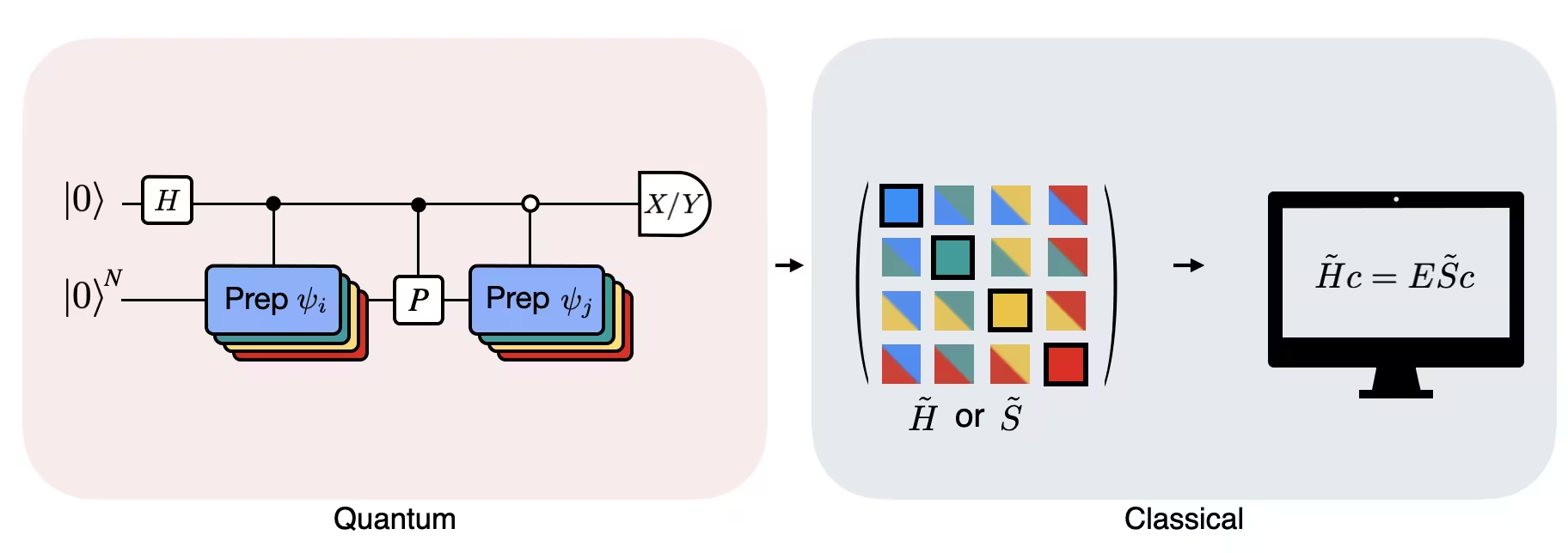
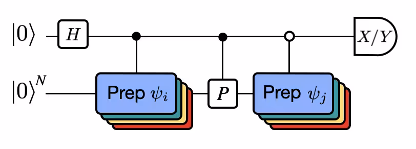
Ipinapakita ng Figure ang circuit representation ng modified Hadamard test, isang paraan na ginagamit upang kalkulahin ang overlap sa pagitan ng iba't ibang quantum state. Para sa bawat matrix element $\tilde{H}_{i,j}$, isinasagawa ang Hadamard test sa pagitan ng state $\vert \psi_i \rangle$, $\vert \psi_j \rangle$. Ito ay naka-highlight sa figure sa pamamagitan ng color scheme para sa mga matrix element at sa kaukulang $\text{Prep} \; \psi_i$, $\text{Prep} \; \psi_j$ operation. Kaya, kailangan ng isang set ng Hadamard test para sa lahat ng posibleng kombinasyon ng mga Krylov space vector upang kalkulahin ang lahat ng matrix element ng projected Hamiltonian $\tilde{H}$. Ang tuktok na wire sa Hadamard test circuit ay isang ancilla qubit na sinusukat sa X o Y basis, ang expectation value nito ay tumutukoy sa halaga ng overlap sa pagitan ng mga state. Ang ibabang wire ay kumakatawan sa lahat ng qubit ng system Hamiltonian. Ang $\text{Prep} \; \psi_i$ operation ay naghahanda ng system qubit sa state $\vert \psi_i \rangle$ na kinokontrol ng state ng ancilla qubit (katulad para sa $\text{Prep} \; \psi_j$) at ang operation $P$ ay kumakatawan sa Pauli decomposition ng system Hamiltonian $H = \sum_i P_i$. Ang mas detalyadong derivation ng mga operation na kinakalkula ng Hadamard test ay ibinigay sa ibaba.

Define Hamiltonian

Isaalang-alang natin ang Heisenberg Hamiltonian para sa $N$ qubit sa linear chain: $H= \sum_{i,j}^N X_i X_j + Y_i Y_j - J Z_i Z_j$

# Define problem Hamiltonian.
n_qubits = 30
J = 1  # coupling strength for ZZ interaction

# Define the Hamiltonian:
H_int = [["I"] * n_qubits for _ in range(3 * (n_qubits - 1))]
for i in range(n_qubits - 1):
    H_int[i][i] = "Z"
    H_int[i][i + 1] = "Z"
for i in range(n_qubits - 1):
    H_int[n_qubits - 1 + i][i] = "X"
    H_int[n_qubits - 1 + i][i + 1] = "X"
for i in range(n_qubits - 1):
    H_int[2 * (n_qubits - 1) + i][i] = "Y"
    H_int[2 * (n_qubits - 1) + i][i + 1] = "Y"
H_int = ["".join(term) for term in H_int]
H_tot = [(term, J) if term.count("Z") == 2 else (term, 1) for term in H_int]

# Get operator
H_op = SparsePauliOp.from_list(H_tot)
print(H_tot)

[('ZZIIIIIIIIIIIIIIIIIIIIIIIIIIII', 1), ('IZZIIIIIIIIIIIIIIIIIIIIIIIIIII', 1), ('IIZZIIIIIIIIIIIIIIIIIIIIIIIIII', 1), ('IIIZZIIIIIIIIIIIIIIIIIIIIIIIII', 1), ('IIIIZZIIIIIIIIIIIIIIIIIIIIIIII', 1), ('IIIIIZZIIIIIIIIIIIIIIIIIIIIIII', 1), ('IIIIIIZZIIIIIIIIIIIIIIIIIIIIII', 1), ('IIIIIIIZZIIIIIIIIIIIIIIIIIIIII', 1), ('IIIIIIIIZZIIIIIIIIIIIIIIIIIIII', 1), ('IIIIIIIIIZZIIIIIIIIIIIIIIIIIII', 1), ('IIIIIIIIIIZZIIIIIIIIIIIIIIIIII', 1), ('IIIIIIIIIIIZZIIIIIIIIIIIIIIIII', 1), ('IIIIIIIIIIIIZZIIIIIIIIIIIIIIII', 1), ('IIIIIIIIIIIIIZZIIIIIIIIIIIIIII', 1), ('IIIIIIIIIIIIIIZZIIIIIIIIIIIIII', 1), ('IIIIIIIIIIIIIIIZZIIIIIIIIIIIII', 1), ('IIIIIIIIIIIIIIIIZZIIIIIIIIIIII', 1), ('IIIIIIIIIIIIIIIIIZZIIIIIIIIIII', 1), ('IIIIIIIIIIIIIIIIIIZZIIIIIIIIII', 1), ('IIIIIIIIIIIIIIIIIIIZZIIIIIIIII', 1), ('IIIIIIIIIIIIIIIIIIIIZZIIIIIIII', 1), ('IIIIIIIIIIIIIIIIIIIIIZZIIIIIII', 1), ('IIIIIIIIIIIIIIIIIIIIIIZZIIIIII', 1), ('IIIIIIIIIIIIIIIIIIIIIIIZZIIIII', 1), ('IIIIIIIIIIIIIIIIIIIIIIIIZZIIII', 1), ('IIIIIIIIIIIIIIIIIIIIIIIIIZZIII', 1), ('IIIIIIIIIIIIIIIIIIIIIIIIIIZZII', 1), ('IIIIIIIIIIIIIIIIIIIIIIIIIIIZZI', 1), ('IIIIIIIIIIIIIIIIIIIIIIIIIIIIZZ', 1), ('XXIIIIIIIIIIIIIIIIIIIIIIIIIIII', 1), ('IXXIIIIIIIIIIIIIIIIIIIIIIIIIII', 1), ('IIXXIIIIIIIIIIIIIIIIIIIIIIIIII', 1), ('IIIXXIIIIIIIIIIIIIIIIIIIIIIIII', 1), ('IIIIXXIIIIIIIIIIIIIIIIIIIIIIII', 1), ('IIIIIXXIIIIIIIIIIIIIIIIIIIIIII', 1), ('IIIIIIXXIIIIIIIIIIIIIIIIIIIIII', 1), ('IIIIIIIXXIIIIIIIIIIIIIIIIIIIII', 1), ('IIIIIIIIXXIIIIIIIIIIIIIIIIIIII', 1), ('IIIIIIIIIXXIIIIIIIIIIIIIIIIIII', 1), ('IIIIIIIIIIXXIIIIIIIIIIIIIIIIII', 1), ('IIIIIIIIIIIXXIIIIIIIIIIIIIIIII', 1), ('IIIIIIIIIIIIXXIIIIIIIIIIIIIIII', 1), ('IIIIIIIIIIIIIXXIIIIIIIIIIIIIII', 1), ('IIIIIIIIIIIIIIXXIIIIIIIIIIIIII', 1), ('IIIIIIIIIIIIIIIXXIIIIIIIIIIIII', 1), ('IIIIIIIIIIIIIIIIXXIIIIIIIIIIII', 1), ('IIIIIIIIIIIIIIIIIXXIIIIIIIIIII', 1), ('IIIIIIIIIIIIIIIIIIXXIIIIIIIIII', 1), ('IIIIIIIIIIIIIIIIIIIXXIIIIIIIII', 1), ('IIIIIIIIIIIIIIIIIIIIXXIIIIIIII', 1), ('IIIIIIIIIIIIIIIIIIIIIXXIIIIIII', 1), ('IIIIIIIIIIIIIIIIIIIIIIXXIIIIII', 1), ('IIIIIIIIIIIIIIIIIIIIIIIXXIIIII', 1), ('IIIIIIIIIIIIIIIIIIIIIIIIXXIIII', 1), ('IIIIIIIIIIIIIIIIIIIIIIIIIXXIII', 1), ('IIIIIIIIIIIIIIIIIIIIIIIIIIXXII', 1), ('IIIIIIIIIIIIIIIIIIIIIIIIIIIXXI', 1), ('IIIIIIIIIIIIIIIIIIIIIIIIIIIIXX', 1), ('YYIIIIIIIIIIIIIIIIIIIIIIIIIIII', 1), ('IYYIIIIIIIIIIIIIIIIIIIIIIIIIII', 1), ('IIYYIIIIIIIIIIIIIIIIIIIIIIIIII', 1), ('IIIYYIIIIIIIIIIIIIIIIIIIIIIIII', 1), ('IIIIYYIIIIIIIIIIIIIIIIIIIIIIII', 1), ('IIIIIYYIIIIIIIIIIIIIIIIIIIIIII', 1), ('IIIIIIYYIIIIIIIIIIIIIIIIIIIIII', 1), ('IIIIIIIYYIIIIIIIIIIIIIIIIIIIII', 1), ('IIIIIIIIYYIIIIIIIIIIIIIIIIIIII', 1), ('IIIIIIIIIYYIIIIIIIIIIIIIIIIIII', 1), ('IIIIIIIIIIYYIIIIIIIIIIIIIIIIII', 1), ('IIIIIIIIIIIYYIIIIIIIIIIIIIIIII', 1), ('IIIIIIIIIIIIYYIIIIIIIIIIIIIIII', 1), ('IIIIIIIIIIIIIYYIIIIIIIIIIIIIII', 1), ('IIIIIIIIIIIIIIYYIIIIIIIIIIIIII', 1), ('IIIIIIIIIIIIIIIYYIIIIIIIIIIIII', 1), ('IIIIIIIIIIIIIIIIYYIIIIIIIIIIII', 1), ('IIIIIIIIIIIIIIIIIYYIIIIIIIIIII', 1), ('IIIIIIIIIIIIIIIIIIYYIIIIIIIIII', 1), ('IIIIIIIIIIIIIIIIIIIYYIIIIIIIII', 1), ('IIIIIIIIIIIIIIIIIIIIYYIIIIIIII', 1), ('IIIIIIIIIIIIIIIIIIIIIYYIIIIIII', 1), ('IIIIIIIIIIIIIIIIIIIIIIYYIIIIII', 1), ('IIIIIIIIIIIIIIIIIIIIIIIYYIIIII', 1), ('IIIIIIIIIIIIIIIIIIIIIIIIYYIIII', 1), ('IIIIIIIIIIIIIIIIIIIIIIIIIYYIII', 1), ('IIIIIIIIIIIIIIIIIIIIIIIIIIYYII', 1), ('IIIIIIIIIIIIIIIIIIIIIIIIIIIYYI', 1), ('IIIIIIIIIIIIIIIIIIIIIIIIIIIIYY', 1)]

Set parameters for the algorithm

Heuristically pumipili tayo ng halaga para sa time-step dt (batay sa upper bound sa Hamiltonian norm). Ang Ref [2] ay nagpakita na ang sapat na maliit na timestep ay $\pi/\vert \vert H \vert \vert$, at mas mainam hanggang sa isang punto na magtantiya ng mas mababang halaga (underestimate) kaysa sa sobrang tantiya, dahil ang sobrang pagtantiya ay maaaring magpahintulot ng mga kontribusyon mula sa high-energy state na masira kahit na ang optimal state sa Krylov space. Sa kabilang banda, ang pagpili ng $dt$ na masyadong maliit ay humahantong sa mas masamang conditioning ng Krylov subspace, dahil ang mga Krylov basis vector ay mas kaunting pagkakaiba mula sa timestep hanggang timestep.

# Get Hamiltonian restricted to single-particle states
single_particle_H = np.zeros((n_qubits, n_qubits))
for i in range(n_qubits):
    for j in range(i + 1):
        for p, coeff in H_op.to_list():
            p_x = Pauli(p).x
            p_z = Pauli(p).z
            if all(
                p_x[k] == ((i == k) + (j == k)) % 2 for k in range(n_qubits)
            ):
                sgn = (
                    (-1j) ** sum(p_z[k] and p_x[k] for k in range(n_qubits))
                ) * ((-1) ** p_z[i])
            else:
                sgn = 0
            single_particle_H[i, j] += sgn * coeff
for i in range(n_qubits):
    for j in range(i + 1, n_qubits):
        single_particle_H[i, j] = np.conj(single_particle_H[j, i])

# Set dt according to spectral norm
dt = np.pi / np.linalg.norm(single_particle_H, ord=2)
dt

np.float64(0.10833078115826875)

At itakda ang iba pang parameter ng algorithm. Para sa layunin ng tutorial na ito, limitahan natin ang ating sarili sa paggamit ng Krylov space na may limang dimension lamang, na medyo nakakahangganan.

# Set parameters for quantum Krylov algorithm
krylov_dim = 5  # size of Krylov subspace
num_trotter_steps = 6
dt_circ = dt / num_trotter_steps

State preparation

Pumili ng reference state $\vert \psi \rangle$ na may overlap sa ground state. Para sa Hamiltonian na ito, ginagamit natin ang state na may excitation sa gitnang qubit $\vert 00..010...00 \rangle$ bilang ating reference state.

qc_state_prep = QuantumCircuit(n_qubits)
qc_state_prep.x(int(n_qubits / 2) + 1)
qc_state_prep.draw("mpl", scale=0.5)

Time evolution

Maaari nating maisakatuparan ang time-evolution operator na nabuo ng ibinigay na Hamiltonian: $U=e^{-iHt}$ sa pamamagitan ng Lie-Trotter approximation.

t = Parameter("t")

## Create the time-evo op circuit
evol_gate = PauliEvolutionGate(
    H_op, time=t, synthesis=LieTrotter(reps=num_trotter_steps)
)

qr = QuantumRegister(n_qubits)
qc_evol = QuantumCircuit(qr)
qc_evol.append(evol_gate, qargs=qr)

<qiskit.circuit.instructionset.InstructionSet at 0x11eef9be0>

Hadamard test

$$\begin{equation*} |0\rangle|0\rangle^N \quad\longrightarrow\quad \frac{1}{\sqrt{2}}\Big(|0\rangle + |1\rangle \Big)|0\rangle^N \quad\longrightarrow\quad \frac{1}{\sqrt{2}}\Big(|0\rangle|0\rangle^N+|1\rangle |\psi_i\rangle\Big) \quad\longrightarrow\quad \frac{1}{\sqrt{2}}\Big(|0\rangle |0\rangle^N+|1\rangle P |\psi_i\rangle\Big) \quad\longrightarrow\quad\frac{1}{\sqrt{2}}\Big(|0\rangle |\psi_j\rangle+|1\rangle P|\psi_i\rangle\Big) \end{equation*}$$

Kung saan ang $P$ ay isa sa mga term sa decomposition ng Hamiltonian $H=\sum P$ at ang $\text{Prep} \; \psi_i$, $\text{Prep} \; \psi_j$ ay mga controlled operation na naghahanda ng $|\psi_i\rangle$, $|\psi_j\rangle$ vector ng unitary Krylov space, na may $|\psi_k\rangle = e^{-i H k dt } \vert \psi \rangle = e^{-i H k dt } U_{\psi} \vert 0 \rangle^N$. Upang sukatin ang $X$, ilapat muna ang $H$...

$$\begin{equation*} \longrightarrow\quad\frac{1}{2}|0\rangle\Big( |\psi_j\rangle + P|\psi_i\rangle\Big) + \frac{1}{2}|1\rangle\Big(|\psi_j\rangle - P|\psi_i\rangle\Big) \end{equation*}$$

... pagkatapos ay sukatin:

$$\begin{equation*} \begin{split} \Rightarrow\quad\langle X\rangle &= \frac{1}{4}\Bigg(\Big\|| \psi_j\rangle + P|\psi_i\rangle \Big\|^2-\Big\||\psi_j\rangle - P|\psi_i\rangle\Big\|^2\Bigg) \\ &= \text{Re}\Big[\langle\psi_j| P|\psi_i\rangle\Big]. \end{split} \end{equation*}$$

Mula sa identity na $|a + b\|^2 = \langle a + b | a + b \rangle = \|a\|^2 + \|b\|^2 + 2\text{Re}\langle a | b \rangle$. Katulad nito, ang pagsukat ng $Y$ ay nagbubunga ng

$$\begin{equation*} \langle Y\rangle = \text{Im}\Big[\langle\psi_j| P|\psi_i\rangle\Big]. \end{equation*}$$

## Create the time-evo op circuit
evol_gate = PauliEvolutionGate(
    H_op, time=dt, synthesis=LieTrotter(reps=num_trotter_steps)
)

## Create the time-evo op dagger circuit
evol_gate_d = PauliEvolutionGate(
    H_op, time=dt, synthesis=LieTrotter(reps=num_trotter_steps)
)
evol_gate_d = evol_gate_d.inverse()

# Put pieces together
qc_reg = QuantumRegister(n_qubits)
qc_temp = QuantumCircuit(qc_reg)
qc_temp.compose(qc_state_prep, inplace=True)
for _ in range(num_trotter_steps):
    qc_temp.append(evol_gate, qargs=qc_reg)
for _ in range(num_trotter_steps):
    qc_temp.append(evol_gate_d, qargs=qc_reg)
qc_temp.compose(qc_state_prep.inverse(), inplace=True)

# Create controlled version of the circuit
controlled_U = qc_temp.to_gate().control(1)

# Create hadamard test circuit for real part
qr = QuantumRegister(n_qubits + 1)
qc_real = QuantumCircuit(qr)
qc_real.h(0)
qc_real.append(controlled_U, list(range(n_qubits + 1)))
qc_real.h(0)

print(
    "Circuit for calculating the real part of the overlap in S via Hadamard test"
)
qc_real.draw("mpl", fold=-1, scale=0.5)

Circuit for calculating the real part of the overlap in S via Hadamard test

Ang Hadamard test circuit ay maaaring maging malalim na circuit kapag na-decompose natin sa native gate (na tataas pa kung isasaalang-alang natin ang topology ng device)

print(
    "Number of layers of 2Q operations",
    qc_real.decompose(reps=2).depth(lambda x: x[0].num_qubits == 2),
)

Number of layers of 2Q operations 112753

Step 2: Optimize problem for quantum hardware execution

Efficient Hadamard test

Maaari nating i-optimize ang malalim na circuit para sa Hadamard test na nakuha natin sa pamamagitan ng pagpapakilala ng ilang approximation at pagsandig sa ilang assumption tungkol sa model Hamiltonian. Halimbawa, isaalang-alang ang sumusunod na circuit para sa Hadamard test:

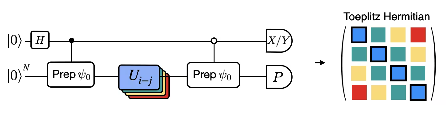
Ipagpalagay natin na maaari nating classically kalkulahin ang $E_0$, ang eigenvalue ng $|0\rangle^N$ sa ilalim ng Hamiltonian $H$. Natutugunan ito kapag ang Hamiltonian ay napapanatili ang U(1) symmetry. Bagaman tila ito ay isang malakas na assumption, may maraming kaso kung saan ligtas na ipagpalagay na may vacuum state (sa kasong ito ay nag-map sa $|0\rangle^N$ state) na hindi naapektuhan ng aksyon ng Hamiltonian. Totoo ito halimbawa para sa chemistry Hamiltonian na naglalarawan ng stable molecule (kung saan ang bilang ng electron ay napapanatili). Dahil ang gate $\text{Prep} \; \psi$, ay naghahanda ng nais na reference state $\ket{psi} = \text{Prep} \; \psi \ket{0} = e^{-i H 0 dt} U_{\psi} \ket{0}$, halimbawa, upang ihanda ang HF state para sa chemistry ang $\text{Prep} \; \psi$ ay magiging produkto ng single-qubit NOT, kaya ang controlled-$\text{Prep} \; \psi$ ay produkto lamang ng CNOT. Pagkatapos ang circuit sa itaas ay nagpapatupad ng sumusunod na state bago ang pagsukat:

$$\begin{equation} \begin{split} \ket{0} \ket{0}^N\xrightarrow{H}&\frac{1}{\sqrt{2}} \left( \ket{0}\ket{0}^N+ \ket{1} \ket{0}^N \right)\\ \xrightarrow{\text{1-ctrl-init}}&\frac{1}{\sqrt{2}}\left(|0\rangle|0\rangle^N+|1\rangle|\psi\rangle\right)\\ \xrightarrow{U}&\frac{1}{\sqrt{2}}\left(e^{i\phi}\ket{0}\ket{0}^N+\ket{1} U\ket{\psi}\right)\\ \xrightarrow{\text{0-ctrl-init}}&\frac{1}{\sqrt{2}} \left( e^{i\phi}\ket{0} \ket{\psi} +\ket{1} U\ket{\psi} \right)\\ =&\frac{1}{2} \left( \ket{+}\left(e^{i\phi}\ket{\psi}+U\ket{\psi}\right) +\ket{-}\left(e^{i\phi}\ket{\psi}-U\ket{\psi}\right) \right)\\ =&\frac{1}{2} \left( \ket{+i}\left(e^{i\phi}\ket{\psi}-iU\ket{\psi}\right) +\ket{-i}\left(e^{i\phi}\ket{\psi}+iU\ket{\psi}\right) \right) \end{split} \end{equation}$$

kung saan ginamit natin ang classical simulable phase shift $U\ket{0}^N = e^{i\phi}\ket{0}^N$ sa ikatlong linya. Kaya ang mga expectation value ay nakukuha bilang

$$\begin{equation} \begin{split} \langle X\otimes P\rangle&=\frac{1}{4} \Big( \left(e^{-i\phi}\bra{\psi}+\bra{\psi}U^\dagger\right)P\left(e^{i\phi}\ket{\psi}+U\ket{\psi}\right) \\ &\qquad-\left(e^{-i\phi}\bra{\psi}-\bra{\psi}U^\dagger\right)P\left(e^{i\phi}\ket{\psi}-U\ket{\psi}\right) \Big)\\ &=\text{Re}\left[e^{-i\phi}\bra{\psi}PU\ket{\psi}\right], \end{split} \end{equation}$$ $$\begin{equation} \begin{split} \langle Y\otimes P\rangle&=\frac{1}{4} \Big( \left(e^{-i\phi}\bra{\psi}+i\bra{\psi}U^\dagger\right)P\left(e^{i\phi}\ket{\psi}-iU\ket{\psi}\right) \\ &\qquad-\left(e^{-i\phi}\bra{\psi}-i\bra{\psi}U^\dagger\right)P\left(e^{i\phi}\ket{\psi}+iU\ket{\psi}\right) \Big)\\ &=\text{Im}\left[e^{-i\phi}\bra{\psi}PU\ket{\psi}\right]. \end{split} \end{equation}$$

Gamit ang mga assumption na ito ay nakayanang natin na isulat ang mga expectation value ng mga operator na kinapapakinabangan na may mas kaunting controlled operation. Sa katunayan, kailangan lang nating ipatupad ang controlled state preparation $\text{Prep} \; \psi$ at hindi controlled time evolution. Ang pag-reframe ng ating pagkalkula gaya ng sa itaas ay magpapahintulot sa atin na malaki ang mabawas sa lalim ng mga resultang circuit.

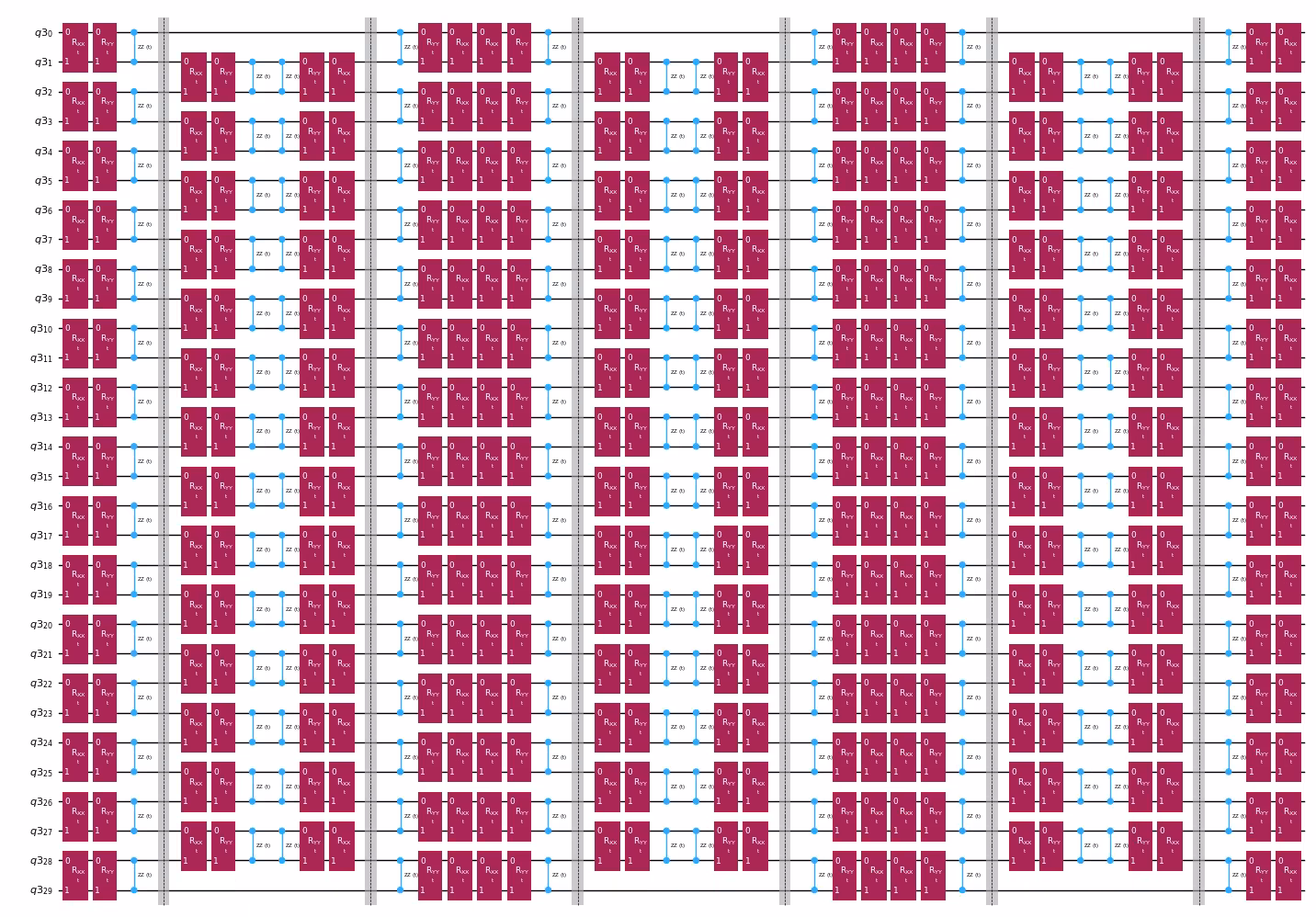
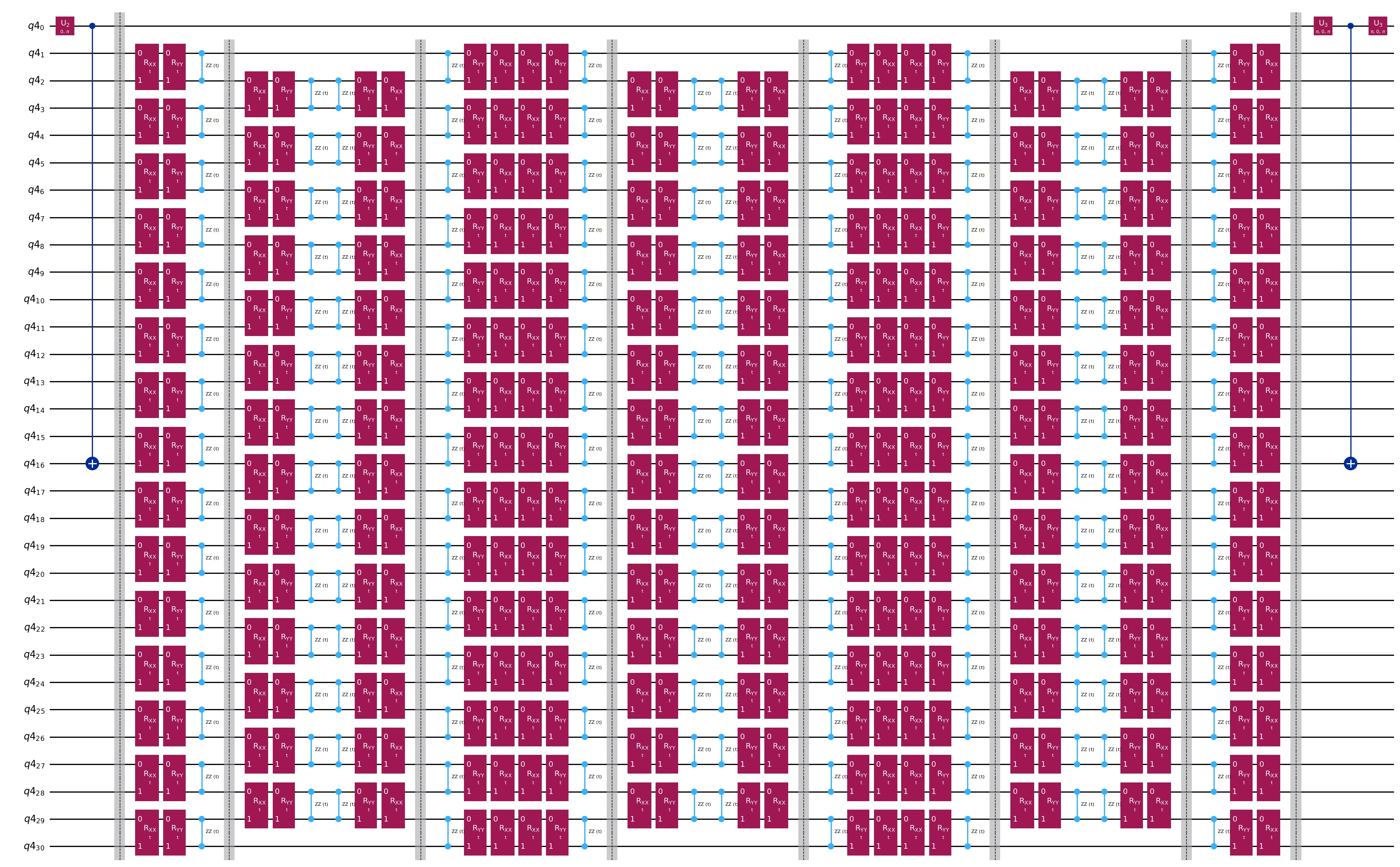
Decompose time-evolution operator with Trotter decomposition

Sa halip na ipatupad nang eksakto ang time-evolution operator, maaari nating gamitin ang Trotter decomposition upang ipatupad ang approximation nito. Ang pag-uulit ng ilang beses sa isang tiyak na order ng Trotter decomposition ay nagbibigay sa atin ng karagdagang pagbabawas ng error na ipinakilala mula sa approximation. Sa sumusunod, direkta naming binubuo ang Trotter implementation sa pinaka-epektibong paraan para sa interaction graph ng Hamiltonian na ating isinasaalang-alang (nearest neighbor interaction lamang). Sa pagsasagawa inilalagay natin ang mga Pauli rotation $R_{xx}$, $R_{yy}$, $R_{zz}$ na may parametrized angle $t$ na kumakatawan sa approximate implementation ng $e^{-i (XX + YY + ZZ) t}$. Dahil sa pagkakaiba sa kahulugan ng mga Pauli rotation at sa time-evolution na sinusubukan nating ipatupad, kailangan nating gamitin ang parameter na $2*dt$ upang makamit ang time-evolution na $dt$. Bukod dito, binabaligtad natin ang order ng mga operation para sa odd number ng mga ulit ng Trotter step, na functionally equivalent ngunit nagpapahintulot na i-synthesize ang magkatabing operation sa isang $SU(2)$ unitary. Ito ay nagbibigay ng mas mababaw na circuit kaysa sa nakuha gamit ang generic PauliEvolutionGate() functionality.

t = Parameter("t")

# Create instruction for rotation about XX+YY-ZZ:
Rxyz_circ = QuantumCircuit(2)
Rxyz_circ.rxx(t, 0, 1)
Rxyz_circ.ryy(t, 0, 1)
Rxyz_circ.rzz(t, 0, 1)
Rxyz_instr = Rxyz_circ.to_instruction(label="RXX+YY+ZZ")

interaction_list = [
    [[i, i + 1] for i in range(0, n_qubits - 1, 2)],
    [[i, i + 1] for i in range(1, n_qubits - 1, 2)],
]  # linear chain

qr = QuantumRegister(n_qubits)
trotter_step_circ = QuantumCircuit(qr)
for i, color in enumerate(interaction_list):
    for interaction in color:
        trotter_step_circ.append(Rxyz_instr, interaction)
    if i < len(interaction_list) - 1:
        trotter_step_circ.barrier()
reverse_trotter_step_circ = trotter_step_circ.reverse_ops()

qc_evol = QuantumCircuit(qr)
for step in range(num_trotter_steps):
    if step % 2 == 0:
        qc_evol = qc_evol.compose(trotter_step_circ)
    else:
        qc_evol = qc_evol.compose(reverse_trotter_step_circ)

qc_evol.decompose().draw("mpl", fold=-1, scale=0.5)

Use an optimized circuit for state preparation

control = 0
excitation = int(n_qubits / 2) + 1
controlled_state_prep = QuantumCircuit(n_qubits + 1)
controlled_state_prep.cx(control, excitation)
controlled_state_prep.draw("mpl", fold=-1, scale=0.5)

Template circuits for calculating matrix elements of $\tilde{S}$ and $\tilde{H}$ via Hadamard test

Ang tanging pagkakaiba sa pagitan ng mga circuit na ginagamit sa Hadamard test ay ang phase sa time-evolution operator at ang mga observable na sinusukat. Kaya maaari tayong maghanda ng template circuit na kumakatawan sa generic circuit para sa Hadamard test, na may mga placeholder para sa mga gate na nakadepende sa time-evolution operator.

# Parameters for the template circuits
parameters = []
for idx in range(1, krylov_dim):
    parameters.append(2 * dt_circ * (idx))

# Create modified hadamard test circuit
qr = QuantumRegister(n_qubits + 1)
qc = QuantumCircuit(qr)
qc.h(0)
qc.compose(controlled_state_prep, list(range(n_qubits + 1)), inplace=True)
qc.barrier()
qc.compose(qc_evol, list(range(1, n_qubits + 1)), inplace=True)
qc.barrier()
qc.x(0)
qc.compose(
    controlled_state_prep.inverse(), list(range(n_qubits + 1)), inplace=True
)
qc.x(0)

qc.decompose().draw("mpl", fold=-1)

print(
    "The optimized circuit has 2Q gates depth: ",
    qc.decompose().decompose().depth(lambda x: x[0].num_qubits == 2),
)

The optimized circuit has 2Q gates depth:  74

Lubhang nabawasan natin ang lalim ng Hadamard test sa pamamagitan ng kombinasyon ng Trotter approximation at uncontrolled unitary

Step 3: Execute using Qiskit primitives

I-instantiate ang backend at itakda ang runtime parameter

service = QiskitRuntimeService()
backend = service.least_busy(operational=True, simulator=False)
if (
    "if_else" not in backend.target.operation_names
):  # Needed as "op_name" could be "if_else"
    backend.target.add_instruction(IfElseOp, name="if_else")
print(backend.name)

Transpiling to a QPU

Una, pumili tayo ng subset ng coupling map na may "magagandang" performing qubit (kung saan ang "maganda" ay medyo arbitrary dito, gusto lamang nating iwasan ang talagang mahinang performing qubit) at lumikha ng bagong target para sa transpilation

target = backend.target
cmap = target.build_coupling_map(filter_idle_qubits=True)
cmap_list = list(cmap.get_edges())

cust_cmap_list = copy.deepcopy(cmap_list)
for q in range(target.num_qubits):
    meas_err = target["measure"][(q,)].error
    t2 = target.qubit_properties[q].t2 * 1e6
    if meas_err > 0.02 or t2 < 100:
        for q_pair in cmap_list:
            if q in q_pair:
                try:
                    cust_cmap_list.remove(q_pair)
                except:
                    continue

for q in cmap_list:
    op_name = list(target.operation_names_for_qargs(q))[0]
    twoq_gate_err = target[f"{op_name}"][q].error
    if twoq_gate_err > 0.005:
        for q_pair in cmap_list:
            if q == q_pair:
                try:
                    cust_cmap_list.remove(q)
                except:
                    continue

cust_cmap = CouplingMap(cust_cmap_list)
cust_target = Target.from_configuration(
    basis_gates=backend.configuration().basis_gates,
    coupling_map=cust_cmap,
)

Pagkatapos ay i-transpile ang virtual circuit sa pinakamahusay na physical layout sa bagong target na ito

basis_gates = list(target.operation_names)
pm = generate_preset_pass_manager(
    optimization_level=3,
    target=cust_target,
    basis_gates=basis_gates,
)

qc_trans = pm.run(qc)

print("depth", qc_trans.depth(lambda x: x[0].num_qubits == 2))
print("num 2q ops", qc_trans.count_ops())
print(
    "physical qubits",
    sorted(
        [
            idx
            for idx, qb in qc_trans.layout.initial_layout.get_physical_bits().items()
            if qb._register.name != "ancilla"
        ]
    ),
)

depth 52
num 2q ops OrderedDict([('rz', 2058), ('sx', 1703), ('cz', 728), ('x', 84), ('barrier', 8)])
physical qubits [91, 92, 93, 94, 95, 98, 99, 108, 109, 110, 111, 113, 114, 115, 119, 127, 132, 133, 134, 135, 137, 139, 147, 148, 149, 150, 151, 152, 153, 154, 155]

Create PUBs for execution with Estimator

# Define observables to measure for S
observable_S_real = "I" * (n_qubits) + "X"
observable_S_imag = "I" * (n_qubits) + "Y"

observable_op_real = SparsePauliOp(
    observable_S_real
)  # define a sparse pauli operator for the observable
observable_op_imag = SparsePauliOp(observable_S_imag)

layout = qc_trans.layout  # get layout of transpiled circuit
observable_op_real = observable_op_real.apply_layout(
    layout
)  # apply physical layout to the observable
observable_op_imag = observable_op_imag.apply_layout(layout)
observable_S_real = (
    observable_op_real.paulis.to_labels()
)  # get the label of the physical observable
observable_S_imag = observable_op_imag.paulis.to_labels()

observables_S = [[observable_S_real], [observable_S_imag]]

# Define observables to measure for H
# Hamiltonian terms to measure
observable_list = []
for pauli, coeff in zip(H_op.paulis, H_op.coeffs):
    # print(pauli)
    observable_H_real = pauli[::-1].to_label() + "X"
    observable_H_imag = pauli[::-1].to_label() + "Y"
    observable_list.append([observable_H_real])
    observable_list.append([observable_H_imag])

layout = qc_trans.layout

observable_trans_list = []
for observable in observable_list:
    observable_op = SparsePauliOp(observable)
    observable_op = observable_op.apply_layout(layout)
    observable_trans_list.append([observable_op.paulis.to_labels()])

observables_H = observable_trans_list

# Define a sweep over parameter values
params = np.vstack(parameters).T

# Estimate the expectation value for all combinations of
# observables and parameter values, where the pub result will have
# shape (# observables, # parameter values).
pub = (qc_trans, observables_S + observables_H, params)

Run circuits

Ang mga circuit para sa $t=0$ ay classically calculable

qc_cliff = qc.assign_parameters({t: 0})

# Get expectation values from experiment
S_expval_real = StabilizerState(qc_cliff).expectation_value(
    Pauli("I" * (n_qubits) + "X")
)
S_expval_imag = StabilizerState(qc_cliff).expectation_value(
    Pauli("I" * (n_qubits) + "Y")
)

# Get expectation values
S_expval = S_expval_real + 1j * S_expval_imag

H_expval = 0
for obs_idx, (pauli, coeff) in enumerate(zip(H_op.paulis, H_op.coeffs)):
    # Get expectation values from experiment
    expval_real = StabilizerState(qc_cliff).expectation_value(
        Pauli(pauli[::-1].to_label() + "X")
    )
    expval_imag = StabilizerState(qc_cliff).expectation_value(
        Pauli(pauli[::-1].to_label() + "Y")
    )
    expval = expval_real + 1j * expval_imag

    # Fill-in matrix elements
    H_expval += coeff * expval

print(H_expval)

(25+0j)

Isagawa ang mga circuit para sa $S$ at $\tilde{H}$ gamit ang Estimator

# Experiment options
num_randomizations = 300
num_randomizations_learning = 30
shots_per_randomization = 100
noise_factors = [1, 1.2, 1.4]
learning_pair_depths = [0, 4, 24, 48]

experimental_opts = {}
experimental_opts["resilience"] = {
    "measure_mitigation": True,
    "measure_noise_learning": {
        "num_randomizations": num_randomizations_learning,
        "shots_per_randomization": shots_per_randomization,
    },
    "zne_mitigation": True,
    "zne": {"noise_factors": noise_factors},
    "layer_noise_learning": {
        "max_layers_to_learn": 10,
        "layer_pair_depths": learning_pair_depths,
        "shots_per_randomization": shots_per_randomization,
        "num_randomizations": num_randomizations_learning,
    },
    "zne": {
        "amplifier": "pea",
        "extrapolated_noise_factors": [0] + noise_factors,
    },
}
experimental_opts["twirling"] = {
    "num_randomizations": num_randomizations,
    "shots_per_randomization": shots_per_randomization,
    "strategy": "all",
}

estimator = Estimator(mode=backend, options=experimental_opts)

job = estimator.run([pub])

Step 4: Post-process and return result in desired classical format

results = job.result()[0]

Calculate Effective Hamiltonian and Overlap matrices

Una ay kalkulahin ang phase na naiipon ng $\vert 0 \rangle$ state sa panahon ng uncontrolled time evolution

prefactors = [
    np.exp(-1j * sum([c for p, c in H_op.to_list() if "Z" in p]) * i * dt)
    for i in range(1, krylov_dim)
]

Kapag mayroon na tayong mga resulta ng circuit execution, maaari nating i-post-process ang data upang kalkulahin ang mga matrix element ng $S$

# Assemble S, the overlap matrix of dimension D:
S_first_row = np.zeros(krylov_dim, dtype=complex)
S_first_row[0] = 1 + 0j

# Add in ancilla-only measurements:
for i in range(krylov_dim - 1):
    # Get expectation values from experiment
    expval_real = results.data.evs[0][0][
        i
    ]  # automatic extrapolated evs if ZNE is used
    expval_imag = results.data.evs[1][0][
        i
    ]  # automatic extrapolated evs if ZNE is used

    # Get expectation values
    expval = expval_real + 1j * expval_imag
    S_first_row[i + 1] += prefactors[i] * expval

S_first_row_list = S_first_row.tolist()  # for saving purposes

S_circ = np.zeros((krylov_dim, krylov_dim), dtype=complex)

# Distribute entries from first row across matrix:
for i, j in it.product(range(krylov_dim), repeat=2):
    if i >= j:
        S_circ[j, i] = S_first_row[i - j]
    else:
        S_circ[j, i] = np.conj(S_first_row[j - i])

Matrix(S_circ)

$$\displaystyle \left[\begin{matrix}1.0 & -0.723052998582984 - 0.345085413575966 i & 0.467051960502366 + 0.516197865254034 i & -0.180546747798251 - 0.492624093654174 i & 0.0012070853532697 + 0.312052218182462 i\\-0.723052998582984 + 0.345085413575966 i & 1.0 & -0.723052998582984 - 0.345085413575966 i & 0.467051960502366 + 0.516197865254034 i & -0.180546747798251 - 0.492624093654174 i\\0.467051960502366 - 0.516197865254034 i & -0.723052998582984 + 0.345085413575966 i & 1.0 & -0.723052998582984 - 0.345085413575966 i & 0.467051960502366 + 0.516197865254034 i\\-0.180546747798251 + 0.492624093654174 i & 0.467051960502366 - 0.516197865254034 i & -0.723052998582984 + 0.345085413575966 i & 1.0 & -0.723052998582984 - 0.345085413575966 i\\0.0012070853532697 - 0.312052218182462 i & -0.180546747798251 + 0.492624093654174 i & 0.467051960502366 - 0.516197865254034 i & -0.723052998582984 + 0.345085413575966 i & 1.0\end{matrix}\right]$$

At ang mga matrix element ng $\tilde{H}$

# Assemble S, the overlap matrix of dimension D:
H_first_row = np.zeros(krylov_dim, dtype=complex)
H_first_row[0] = H_expval

for obs_idx, (pauli, coeff) in enumerate(zip(H_op.paulis, H_op.coeffs)):
    # Add in ancilla-only measurements:
    for i in range(krylov_dim - 1):
        # Get expectation values from experiment
        expval_real = results.data.evs[2 + 2 * obs_idx][0][
            i
        ]  # automatic extrapolated evs if ZNE is used
        expval_imag = results.data.evs[2 + 2 * obs_idx + 1][0][
            i
        ]  # automatic extrapolated evs if ZNE is used

        # Get expectation values
        expval = expval_real + 1j * expval_imag
        H_first_row[i + 1] += prefactors[i] * coeff * expval

H_first_row_list = H_first_row.tolist()

H_eff_circ = np.zeros((krylov_dim, krylov_dim), dtype=complex)

# Distribute entries from first row across matrix:
for i, j in it.product(range(krylov_dim), repeat=2):
    if i >= j:
        H_eff_circ[j, i] = H_first_row[i - j]
    else:
        H_eff_circ[j, i] = np.conj(H_first_row[j - i])

Matrix(H_eff_circ)

$$\displaystyle \left[\begin{matrix}25.0 & -14.2437089383409 - 6.50486277982165 i & 10.2857217968584 + 9.0431912203186 i & -5.15587257589417 - 8.88280836036843 i & 1.98818301405581 + 5.8897614762563 i\\-14.2437089383409 + 6.50486277982165 i & 25.0 & -14.2437089383409 - 6.50486277982165 i & 10.2857217968584 + 9.0431912203186 i & -5.15587257589417 - 8.88280836036843 i\\10.2857217968584 - 9.0431912203186 i & -14.2437089383409 + 6.50486277982165 i & 25.0 & -14.2437089383409 - 6.50486277982165 i & 10.2857217968584 + 9.0431912203186 i\\-5.15587257589417 + 8.88280836036843 i & 10.2857217968584 - 9.0431912203186 i & -14.2437089383409 + 6.50486277982165 i & 25.0 & -14.2437089383409 - 6.50486277982165 i\\1.98818301405581 - 5.8897614762563 i & -5.15587257589417 + 8.88280836036843 i & 10.2857217968584 - 9.0431912203186 i & -14.2437089383409 + 6.50486277982165 i & 25.0\end{matrix}\right]$$

Sa wakas, maaari nating lutasin ang generalized eigenvalue problem para sa $\tilde{H}$:

$\tilde{H} \vec{c} = c S \vec{c}$

at makakuha ng estimate ng ground state energy $c_{min}$

gnd_en_circ_est_list = []
for d in range(1, krylov_dim + 1):
    # Solve generalized eigenvalue problem for different size of the Krylov space
    gnd_en_circ_est = solve_regularized_gen_eig(
        H_eff_circ[:d, :d], S_circ[:d, :d], threshold=9e-1
    )
    gnd_en_circ_est_list.append(gnd_en_circ_est)
    print("The estimated ground state energy is: ", gnd_en_circ_est)

The estimated ground state energy is:  25.0
The estimated ground state energy is:  22.572154819954875
The estimated ground state energy is:  21.691509219286587
The estimated ground state energy is:  21.23882298756386
The estimated ground state energy is:  20.965499325470294

Para sa single-particle sector, maaari tayong epektibong kalkulahin ang ground state ng sector na ito ng Hamiltonian sa classical

gs_en = single_particle_gs(H_op, n_qubits)

n_sys_qubits 30
n_exc 1 , subspace dimension 31
single particle ground state energy:  21.021912418526906

plt.plot(
    range(1, krylov_dim + 1),
    gnd_en_circ_est_list,
    color="blue",
    linestyle="-.",
    label="KQD estimate",
)
plt.plot(
    range(1, krylov_dim + 1),
    [gs_en] * krylov_dim,
    color="red",
    linestyle="-",
    label="exact",
)
plt.xticks(range(1, krylov_dim + 1), range(1, krylov_dim + 1))
plt.legend()
plt.xlabel("Krylov space dimension")
plt.ylabel("Energy")
plt.title(
    "Estimating Ground state energy with Krylov Quantum Diagonalization"
)
plt.show()

Appendix: Krylov subspace from real time-evolutions

Ang unitary Krylov space ay tinukoy bilang

$$\mathcal{K}_U(H, |\psi\rangle) = \text{span}\left\{ |\psi\rangle, e^{-iH\,dt} |\psi\rangle, \dots, e^{-irH\,dt} |\psi\rangle \right\}$$

para sa ilang timestep $dt$ na tutukuyin natin mamaya. Panandaliang ipagpalagay na ang $r$ ay even: kung gayon ay tukuyin ang $d=r/2$. Pansinin na kapag ini-project natin ang Hamiltonian sa Krylov space sa itaas, ito ay hindi mapagkakaila mula sa Krylov space

$$\mathcal{K}_U(H, |\psi\rangle) = \text{span}\left\{ e^{i\,d\,H\,dt}|\psi\rangle, e^{i(d-1)H\,dt} |\psi\rangle, \dots, e^{-i(d-1)H\,dt} |\psi\rangle, e^{-i\,d\,H\,dt} |\psi\rangle \right\},$$

ibig sabihin, kung saan ang lahat ng time-evolution ay na-shift pabalik ng $d$ timestep. Ang dahilan kung bakit ito ay hindi mapagkakaila ay dahil ang mga matrix element

$$\tilde{H}_{j,k} = \langle\psi|e^{i\,j\,H\,dt}He^{-i\,k\,H\,dt}|\psi\rangle=\langle\psi|He^{i(j-k)H\,dt}|\psi\rangle$$

ay invariant sa ilalim ng overall shift ng evolution time, dahil ang mga time-evolution ay commute sa Hamiltonian. Para sa odd $r$, maaari nating gamitin ang analysis para sa $r-1$.

Gusto nating ipakita na saanman sa Krylov space na ito, may garantisadong low-energy state. Ginagawa natin ito sa pamamagitan ng sumusunod na resulta, na hinango mula sa Theorem 3.1 sa [3]:

Claim 1: mayroong function $f$ na para sa mga energy $E$ sa spectral range ng Hamiltonian (ibig sabihin, sa pagitan ng ground state energy at ng maximum energy)...

1. $f(E_0)=1$
2. $|f(E)|\le2\left(1 + \delta\right)^{-d}$ para sa lahat ng halaga ng $E$ na nakahiwalay ng $\ge\delta$ mula sa $E_0$, ibig sabihin, ito ay exponentially suppressed
3. Ang $f(E)$ ay isang linear combination ng $e^{ijE\,dt}$ para sa $j=-d,-d+1,...,d-1,d$

Nagbibigay tayo ng patunay sa ibaba, ngunit maaari itong ligtas na laktawan maliban kung nais mong maunawaan ang buong, mahigpit na argumento. Sa ngayon nakatuon tayo sa mga implikasyon ng claim sa itaas. Sa pamamagitan ng property 3 sa itaas, makikita natin na ang shifted Krylov space sa itaas ay naglalaman ng state $f(H)|\psi\rangle$. Ito ang ating low-energy state. Upang makita kung bakit, isulat ang $|\psi\rangle$ sa energy eigenbasis:

$$|\psi\rangle = \sum_{k=0}^{N}\gamma_k|E_k\rangle,$$

kung saan ang $|E_k\rangle$ ay ang kth energy eigenstate at ang $\gamma_k$ ay ang amplitude nito sa initial state $|\psi\rangle$. Ipinahayag sa mga termino nito, ang $f(H)|\psi\rangle$ ay ibinigay ng

$$f(H)|\psi\rangle = \sum_{k=0}^{N}\gamma_kf(E_k)|E_k\rangle,$$

gamit ang katotohanan na maaari nating palitan ang $H$ ng $E_k$ kapag ito ay kumikilos sa eigenstate $|E_k\rangle$. Ang energy error ng state na ito ay samakatuwid

$$\text{energy error} = \frac{\langle\psi|f(H)(H-E_0)f(H)|\psi\rangle}{\langle\psi|f(H)^2|\psi\rangle}$$ $$= \frac{\sum_{k=0}^{N}|\gamma_k|^2f(E_k)^2(E_k-E_0)}{\sum_{k=0}^{N}|\gamma_k|^2f(E_k)^2}.$$

Upang gawing upper bound na mas madaling maunawaan, una ay ihiwalay natin ang sum sa numerator sa mga term na may $E_k-E_0\le\delta$ at mga term na may $E_k-E_0>\delta$:

$$\text{energy error} = \frac{\sum_{E_k\le E_0+\delta}|\gamma_k|^2f(E_k)^2(E_k-E_0)}{\sum_{k=0}^{N}|\gamma_k|^2f(E_k)^2} + \frac{\sum_{E_k> E_0+\delta}|\gamma_k|^2f(E_k)^2(E_k-E_0)}{\sum_{k=0}^{N}|\gamma_k|^2f(E_k)^2}.$$

Maaari nating i-upper bound ang unang term ng $\delta$,

$$\frac{\sum_{E_k\le E_0+\delta}|\gamma_k|^2f(E_k)^2(E_k-E_0)}{\sum_{k=0}^{N}|\gamma_k|^2f(E_k)^2} < \frac{\delta\sum_{E_k\le E_0+\delta}|\gamma_k|^2f(E_k)^2}{\sum_{k=0}^{N}|\gamma_k|^2f(E_k)^2} \le \delta,$$

kung saan ang unang hakbang ay sumusunod dahil $E_k-E_0\le\delta$ para sa bawat $E_k$ sa sum, at ang pangalawang hakbang ay sumusunod dahil ang sum sa numerator ay isang subset ng sum sa denominator. Para sa pangalawang term, una ay i-lower bound natin ang denominator ng $|\gamma_0|^2$, dahil $f(E_0)^2=1$: ang pagdagdag ng lahat pabalik, ito ay nagbibigay ng

$$\text{energy error} \le \delta + \frac{1}{|\gamma_0|^2}\sum_{E_k>E_0+\delta}|\gamma_k|^2f(E_k)^2(E_k-E_0).$$

Upang pasimplehin ang natitira, pansinin na para sa lahat ng $E_k$ na ito, sa pamamagitan ng kahulugan ng $f$ alam natin na $f(E_k)^2 \le 4\left(1 + \delta\right)^{-2d}$. Bukod pa sa pag-upper bound ng $E_k-E_0<2\|H\|$ at pag-upper bound ng $\sum_{E_k>E_0+\delta}|\gamma_k|^2<1$ ay nagbibigay ng

$$\text{energy error} \le \delta + \frac{8}{|\gamma_0|^2}\|H\|\left(1 + \delta\right)^{-2d}.$$

Ito ay totoo para sa anumang $\delta>0$, kaya kung itakda natin ang $\delta$ na katumbas ng ating layuning error, kung gayon ang error bound sa itaas ay umabot sa exponentially sa Krylov dimension $2d=r$. Pansinin din na kung $\delta<E_1-E_0$ kung gayon ang $\delta$ term ay talagang nawawala sa bound sa itaas.

Upang kumpletuhin ang argumento, una ay pansinin natin na ang nasa itaas ay ang energy error lamang ng partikular na state $f(H)|\psi\rangle$, sa halip na ang energy error ng pinakamababang energy state sa Krylov space. Gayunpaman, sa pamamagitan ng (Rayleigh-Ritz) variational principle, ang energy error ng pinakamababang energy state sa Krylov space ay upper bounded ng energy error ng anumang state sa Krylov space, kaya ang nasa itaas ay isa ring upper bound sa energy error ng pinakamababang energy state, ibig sabihin, ang output ng Krylov quantum diagonalization algorithm.

Ang katulad na analysis gaya ng sa itaas ay maaaring isagawa na kasama pa ang noise at ang thresholding procedure na tinalakay sa notebook. Tingnan ang [2] at [4] para sa analysis na ito.

Appendix: proof of Claim 1

Ang sumusunod ay karamihan ay hinango mula sa [3], Theorem 3.1: hayaan ang $0 < a < b$ at hayaan ang $\Pi^*_d$ na maging space ng residual polynomial (polynomial na ang halaga sa 0 ay 1) na may degree na hindi hihigit sa $d$. Ang solusyon sa

$$\beta(a, b, d) = \min_{p \in \Pi^*_d} \max_{x \in [a, b]} |p(x)| \quad$$

ay

$$p^*(x) = \frac{T_d\left(\frac{b + a - 2x}{b - a}\right)}{T_d\left(\frac{b + a}{b - a}\right)}, \quad$$

at ang kaukulang minimal value ay

$$\beta(a, b, d) = T_d^{-1}\left(\frac{b + a}{b - a}\right).$$

Gusto nating i-convert ito sa isang function na maaaring ipahayag nang natural sa mga termino ng complex exponential, dahil iyon ang mga tunay na time-evolution na bumubuo ng quantum Krylov space. Upang gawin ito, maginhawa na ipakilala ang sumusunod na transformation ng mga energy sa loob ng spectral range ng Hamiltonian sa mga numero sa range na $[0,1]$: tukuyin

$$g(E) = \frac{1-\cos\big((E-E_0)dt\big)}{2},$$

kung saan ang $dt$ ay isang timestep na $-\pi < E_0dt < E_\text{max}dt < \pi$. Pansinin na $g(E_0)=0$ at ang $g(E)$ ay lumalaki habang ang $E$ ay lumilipat palayo sa $E_0$.

Ngayon gamit ang polynomial $p^*(x)$ na may parameter a, b, d na itinakda sa $a = g(E_0 + \delta)$, $b = 1$, at d = int(r/2), tinutukoy natin ang function:

$$f(E) = p^* \left( g(E) \right) = \frac{T_d\left(1 + 2\frac{\cos\big((E-E_0)dt\big) - \cos\big(\delta\,dt\big)}{1 +\cos\big(\delta\,dt\big)}\right)}{T_d\left(1 + 2\frac{1-\cos\big(\delta\,dt\big)}{1 + \cos\big(\delta\,dt\big)}\right)}$$

kung saan ang $E_0$ ay ang ground state energy. Makikita natin sa pamamagitan ng pag-insert ng $\cos(x)=\frac{e^{ix}+e^{-ix}}{2}$ na ang $f(E)$ ay isang trigonometric polynomial ng degree $d$, ibig sabihin, isang linear combination ng $e^{ijE\,dt}$ para sa $j=-d,-d+1,...,d-1,d$. Bukod pa rito, mula sa kahulugan ng $p^*(x)$ sa itaas mayroon tayong $f(E_0)=p(0)=1$ at para sa anumang $E$ sa spectral range na $\vert E-E_0 \vert > \delta$ mayroon tayo

$$|f(E)| \le \beta(a, b, d) = T_d^{-1}\left(1 + 2\frac{1-\cos\big(\delta\,dt\big)}{1 + \cos\big(\delta\,dt\big)}\right)$$ $$\leq 2\left(1 + \delta\right)^{-d} = 2\left(1 + \delta\right)^{-\lfloor k/2\rfloor}.$$

References

[1] N. Yoshioka, M. Amico, W. Kirby et al. "Diagonalization of large many-body Hamiltonians on a quantum processor". arXiv:2407.14431

[2] Ethan N. Epperly, Lin Lin, and Yuji Nakatsukasa. "A theory of quantum subspace diagonalization". SIAM Journal on Matrix Analysis and Applications 43, 1263–1290 (2022).

[3] Å. Björck. "Numerical methods in matrix computations". Texts in Applied Mathematics. Springer International Publishing. (2014).

[4] William Kirby. "Analysis of quantum Krylov algorithms with errors". Quantum 8, 1457 (2024).

Tutorial survey

Mangyaring sagutan ang maikling survey na ito upang magbigay ng feedback tungkol sa tutorial na ito. Ang iyong mga insight ay makakatulong sa amin na mapabuti ang aming mga alok sa nilalaman at karanasan ng user.

Link sa survey

Note: This survey is provided by IBM Quantum and relates to the original English content. To give feedback on doQumentation's website, translations, or code execution, please open a GitHub issue.