Pauli correlation encoding upang Bawasan ang Pangangailangan sa max-cut

Pagtantya ng paggamit: 35 minuto sa isang Eagle r3 processor (PAALALA: Ito ay isang tantya lamang. Maaaring mag-iba ang iyong runtime.)

Mga Resulta ng Pagkatuto

Pagkatapos ng tutorial na ito, inaasahang magkakaroon ang mga gumagamit ng sumusunod na mga kinalabasan:

Maunawaan ang mga teoretikal na prinsipyo ng Pauli Correlation Encoding (PCE), kasama ang kung paano nagbibigay-daan ang multi‑body Pauli string sa polynomial compression ng mga classical optimization problem.
Maipatupad ang PCE sa praktis upang ma-encode at malutas ang mga large‑scale optimization task sa near‑term quantum hardware.

Mga Paunang Kaalaman

Inirerekomenda naming makilala muna ang mga sumusunod na paksa bago simulan ang tutorial na ito:

Konteksto

Ang tutorial na ito ay nagpapakita ng Pauli Correlation Encoding (PCE) [1], isang diskarte na idinisenyo upang mag-encode ng mga optimization problem sa mga qubit nang mas maayos para sa quantum computation. Ang PCE ay nagmamapa ng mga classical variable sa optimization problem tungo sa multi-body Pauli-matrix correlation, na nagreresulta sa polynomial compression ng space requirement ng problema. Sa pamamagitan ng paggamit ng PCE, ang bilang ng mga qubit na kailangan para sa pag-encode ay nabababawasan, na ginagawang partikular na kapaki-pakinabang ito para sa near-term quantum device na may limitadong qubit resource. Dagdag pa, napatunayan sa pamamagitan ng analytical method na ang PCE ay likas na nakakabawas ng barren plateau, na nag-aalok ng super-polynomial resilience laban sa phenomenong ito. Ang built-in na feature na ito ay nagpapahintulot ng walang kapantay na performance sa mga quantum optimization solver.

Pangkalahatang-ideya

Ang PCE approach ay binubuo ng tatlong pangunahing hakbang, gaya ng ipinakikita sa Figure 1 mula sa [1] sa ibaba:

Pag-encode ng optimization problem tungo sa isang Pauli correlation space.
Paglutas ng problema gamit ang quantum-classical optimization solver.
Pag-decode ng solusyon pabalik sa orihinal na optimization space. Ang PCE approach ay maaaring iangkop sa anumang quantum optimization solver na may kakayahang magproseso ng mga Pauli correlation matrix. 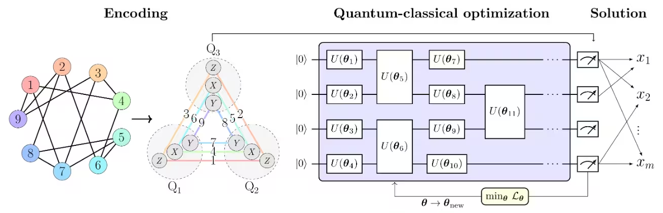Sa Figure 1 mula sa [1], ang problema ng max-cut ay ginagamit bilang halimbawa upang ilarawan ang PCE approach. Ang max-cut problem na may $m=9$ node ay ine-encode tungo sa isang Pauli correlation space, na kumakatawan sa optimization problem bilang correlation matrix — partikular na, two-body Pauli-matrix correlation sa $n=3$ qubit $(Q_1, Q_2, Q_3)$ . Ang mga kulay ng node ay nagsasaad ng Pauli string na ginagamit para sa bawat naka-encode na node. Halimbawa, ang node 1, na tumutugma sa binary variable $x_1$ , ay ine-encode sa pamamagitan ng expectation value ng $Z_1 \otimes Z_2 \otimes I_3$ , habang ang $x_8$ ay ine-encode ng $I_1 \otimes Y_2 \otimes Y_3$ . Ito ay tumutugma sa pag-compress ng $m$ variable ng problema tungo sa $n = O(m^{1/2})$ qubit. Sa mas malawak na pag-unawa, ang $k$ -body correlation ay nagpapahintulot ng polynomial compression na may order na $k$ , na may $k>1$ . Ang napiling Pauli set ay binubuo ng tatlong subset ng mutually-commuting Pauli string, na nagpapahintulot na ang lahat ng $m$ correlation ay matantya nang eksperimental gamit lamang ang tatlong measurement setting.

Ang isang loss function $\mathcal{L}$ ng mga Pauli expectation value na gumagaya sa orihinal na max-cut objective function ay ginagawa. Pagkatapos, ang loss function ay ino-optimize gamit ang quantum-classical optimization solver, gaya ng Variational Quantum Eigensolver (VQE).

Kapag natapos na ang optimization, ang solusyon ay dine-decode pabalik sa orihinal na optimization space, na nagbubunga ng optimal na max-cut solution.

Mga Pangangailangan

Bago simulan ang tutorial na ito, tiyaking mayroon kayo ng sumusunod na naka-install:

Qiskit SDK v1.0 o mas bago, na may visualization support
Qiskit Runtime v0.22 o mas bago (pip install qiskit-ibm-runtime)

Pag-setup

# Added by doQumentation — required packages for this notebook
!pip install -q networkx numpy qiskit qiskit-aer qiskit-ibm-runtime rustworkx scipy

from itertools import combinations

import numpy as np
import rustworkx as rx
import networkx as nx

from scipy.optimize import minimize, OptimizeResult

from qiskit.circuit.library import efficient_su2
from qiskit.transpiler.preset_passmanagers import generate_preset_pass_manager
from qiskit.quantum_info import SparsePauliOp
from qiskit_ibm_runtime import EstimatorV2 as Estimator
from qiskit_ibm_runtime import QiskitRuntimeService
from qiskit_ibm_runtime import Session
from rustworkx.visualization import mpl_draw
from qiskit_aer import AerSimulator

def calc_cut_size(graph, partition0, partition1):
    """Calculate the cut size of the given partitions of the graph."""

    cut_size = 0
    for edge0, edge1 in graph.edge_list():
        if edge0 in partition0 and edge1 in partition1:
            cut_size += 1
        elif edge0 in partition1 and edge1 in partition0:
            cut_size += 1
    return cut_size

Maliit na Halimbawa sa Simulator

service = QiskitRuntimeService()
real_backend = service.least_busy(
    operational=True, simulator=False, min_num_qubits=156
)
backend = AerSimulator.from_backend(real_backend)
print(f"We are using the {backend.name}")

We are using the aer_simulator_from(ibm_pittsburgh)

Hakbang 1: Mag-map ng Mga Classical Input tungo sa Quantum Problem

Ang max-cut problem

Ang max-cut problem ay isang combinatorial optimization problem na tinukoy sa isang graph $G = (V, E)$ , kung saan ang $V$ ay ang set ng mga vertex at ang $E$ ay ang set ng mga edge. Ang layunin ay hatiin ang mga vertex tungo sa dalawang set, $S$ at $V \setminus S$ , sa paraang ang bilang ng mga edge sa pagitan ng dalawang set ay napapalaki. Para sa detalyadong paglalarawan ng max-cut problem, pakitingin ang tutorial na Quantum approximate optimization algorithm. Ang max-cut problem ay ginagamit din bilang halimbawa sa tutorial na Advanced techniques for QAOA. Sa mga tutorial na iyon, ang QAOA algorithm ay ginagamit upang lutasin ang max-cut problem.

Graph -> Hamiltonian

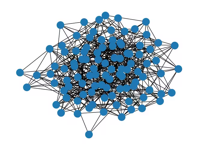
Una nating isaalang-alang ang isang random graph na may 100 node.

num_nodes = 100  # Number of nodes in graph
seed = 42
graph = rx.undirected_gnp_random_graph(num_nodes, 0.1, seed=seed)
mpl_draw(graph)

Output of the previous code cell

nx_graph = nx.Graph()
nx_graph.add_nodes_from(range(num_nodes))

for edge in graph.edge_list():
    nx_graph.add_edge(edge[0], edge[1])

curr_cut_size, partition = nx.approximation.one_exchange(nx_graph, seed=1)
print(f"Initial cut size: {curr_cut_size}")

Initial cut size: 345

Ine-encode natin ang graph na may 100 node tungo sa two-body Pauli-matrix correlation sa siyam na qubit (tingnan ang paliwanag sa ibaba). Ang graph ay kinakatawan bilang correlation matrix, kung saan ang bawat node ay ine-encode ng isang Pauli string. Ang sign ng expectation value ng Pauli string ay nagsasaad ng partition ng node. Halimbawa, ang node 0 ay ine-encode ng isang Pauli string, $\prod_0 = I_{8} \otimes ... I_2 \otimes X_1 \otimes X_0$ . Ang sign ng expectation value ng Pauli string na ito ay nagsasaad ng partition ng node 0. Tinutukoy natin ang Pauli-correlation encoding (PCE) na nauukol sa $\prod$ bilang

$x_i \coloneqq \textit{sgn}(\langle\prod_i \rangle),$

kung saan ang $x_i$ ay ang partition ng node $i$ at ang $\langle \prod_i \rangle \coloneqq \langle \psi |\prod_i| \psi \rangle$ ay ang expectation value ng Pauli string na nag-eencode ng node $i$ sa isang quantum state na $|\psi \rangle$ . Ngayon, i-encode natin ang graph tungo sa isang Hamiltonian gamit ang PCE. Hinahati natin ang mga node tungo sa tatlong set: $S_1$ , $S_2$ , at $S_3$ . Pagkatapos, ine-encode natin ang mga node sa bawat set gamit ang mga Pauli string na may $X$ , $Y$ , at $Z$ , ayon sa pagkakabanggit. Kailangan nating makuha ang relasyon sa pagitan ng bilang ng mga node at qubit na kailangan natin upang ma-encode ang lahat ng node. Ang paggamit ng lahat ng posibleng permutasyon para sa encoding ay nagbibigay ng:

m=3\binom{n}{k}.

Sa halimbawang ito, isinasaalang-alang natin ang $k=2$ , kaya,

m = \frac{3}{2} n(n-1).

Samakatuwid, ang bilang ng qubit na $n$ na kailangan upang ipahayag ang isang tiyak na bilang ng node na $m$ ay:

n = \left\lceil \frac{1 + \sqrt{1 + \tfrac{8}{3}m}}{2} \right\rceil.

Tandaan na ang simbolong $\lceil \cdot \rceil$ ay kumakatawan sa ceiling function, na inaangat ang anumang real number pataas sa susunod na integer. Tinitiyak nito na ang bilang ng qubit ay isang integer.

num_qubits = int(np.ceil((1 + np.sqrt(1 + (8 / 3) * num_nodes)) / 2))

list_size = num_nodes // 3
node_x = [i for i in range(list_size)]
node_y = [i for i in range(list_size, 2 * list_size)]
node_z = [i for i in range(2 * list_size, num_nodes)]

print(f"Number of qubits: {num_qubits}")
print("List 1:", node_x)
print("List 2:", node_y)
print("List 3:", node_z)

Number of qubits: 9
List 1: [0, 1, 2, 3, 4, 5, 6, 7, 8, 9, 10, 11, 12, 13, 14, 15, 16, 17, 18, 19, 20, 21, 22, 23, 24, 25, 26, 27, 28, 29, 30, 31, 32]
List 2: [33, 34, 35, 36, 37, 38, 39, 40, 41, 42, 43, 44, 45, 46, 47, 48, 49, 50, 51, 52, 53, 54, 55, 56, 57, 58, 59, 60, 61, 62, 63, 64, 65]
List 3: [66, 67, 68, 69, 70, 71, 72, 73, 74, 75, 76, 77, 78, 79, 80, 81, 82, 83, 84, 85, 86, 87, 88, 89, 90, 91, 92, 93, 94, 95, 96, 97, 98, 99]

def build_pauli_correlation_encoding(pauli, node_list, n, k=2):
    pauli_correlation_encoding = []
    for idx, c in enumerate(combinations(range(n), k)):
        if idx >= len(node_list):
            break
        paulis = ["I"] * n
        paulis[c[0]], paulis[c[1]] = pauli, pauli
        pauli_correlation_encoding.append(("".join(paulis)[::-1], 1))

    hamiltonian = []
    for pauli, weight in pauli_correlation_encoding:
        hamiltonian.append(SparsePauliOp.from_list([(pauli, weight)]))

    return hamiltonian

pauli_correlation_encoding_x = build_pauli_correlation_encoding(
    "X", node_x, num_qubits
)
pauli_correlation_encoding_y = build_pauli_correlation_encoding(
    "Y", node_y, num_qubits
)
pauli_correlation_encoding_z = build_pauli_correlation_encoding(
    "Z", node_z, num_qubits
)

Hakbang 2: I-optimize ang Problema para sa Quantum Hardware Execution

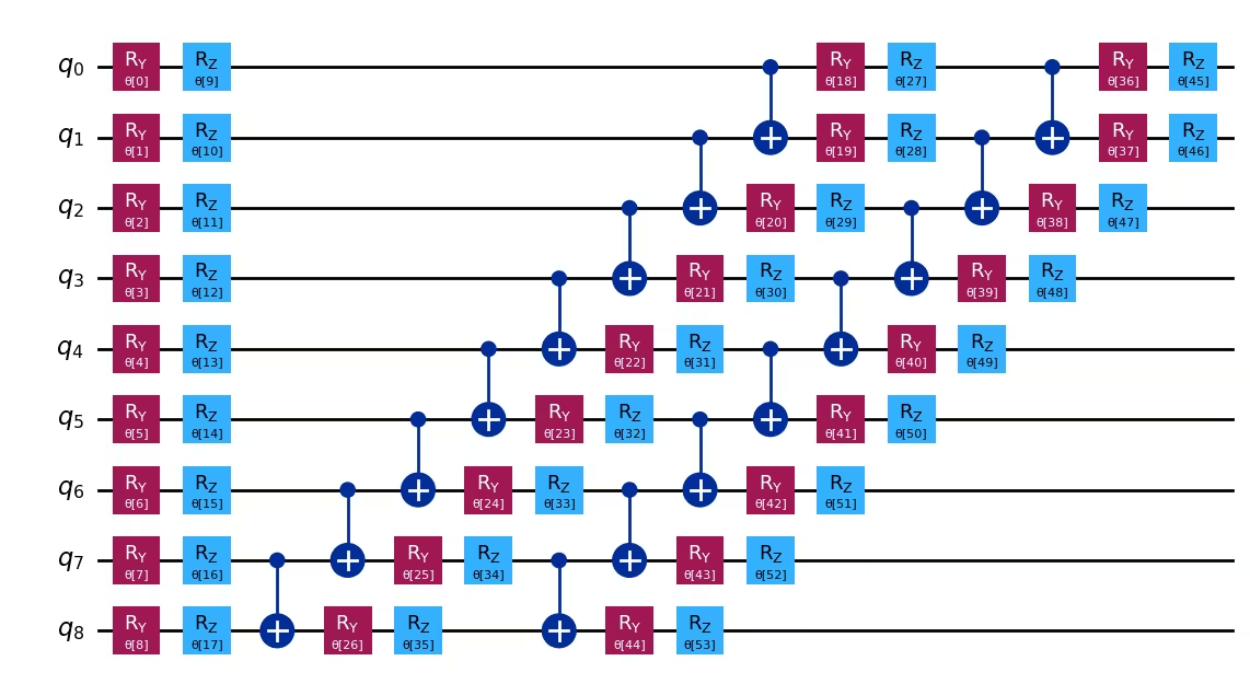
Quantum circuit

Dito, ang state na $|\psi \rangle$ ay may parameter na $\mathbf{\theta}$ , at ino-optimize natin ang mga parameter na $\mathbf{\theta}$ na ito gamit ang variational approach. Ang tutorial na ito ay gumagamit ng efficient_su2 ansatz para sa ating variational algorithm dahil sa expressive capability at kadaling i-implement nito. Ginagamit din natin ang relaxed loss function, na ipapakita pa sa tutorial na ito. Bilang resulta, makakayanan nating lutasin ang mga large-scale problem gamit ang mas kaunting qubit at mas mababaw na circuit depth.

# Build the quantum circuit
qc = efficient_su2(num_qubits, su2_gates=["ry", "rz"], reps=2)
qc.draw("mpl")

Output of the previous code cell

# Optimize the circuit

pm = generate_preset_pass_manager(optimization_level=3, backend=backend)
qc = pm.run(qc)

Loss function

Para sa loss function na $\mathcal{L}$ , gumagamit tayo ng relaxation ng max-cut objective function gaya ng inilarawan sa [1], na tinutukoy bilang $\mathcal{V}(\mathbf{x}) \coloneqq \sum_{(i, j) \in E} W_{i, j}(1-x_i x_j)$ . Dito, ang $W_{i, j}$ ay nagsasaad ng weight ng edge na $(i, j)$ , at ang $x_i$ ay kumakatawan sa partition ng node $i$ . Ang loss function na $\mathcal{L}$ ay ibinibigay sa pamamagitan ng:

$\mathcal{L}\coloneqq \sum_{(i, j) \in E} W_{i, j} \text{tanh} (\alpha \langle\prod_i \rangle) \text{tanh} (\alpha \langle\prod_j \rangle) + \mathcal{L}^{(\text{reg})},$

kung saan ang max-cut objective function ay pinalitan ng smooth hyperbolic tangent ng mga expectation value ng mga Pauli string na nag-eencode sa mga node. Ang regularization term na $\mathcal{L}^{(\text{reg})}$ at ang rescaling factor na $\alpha$ , na proporsyonal sa bilang ng mga qubit, ay ipinakilala upang mapabuti ang performance ng solver.

Ang regularization term ay tinutukoy bilang:

Ang $\mathcal{L}^{(\text{reg})}$ ay tinutukoy bilang $\mathcal{L}^{(\text{reg})} \coloneqq \beta \nu \lbrack \frac{1}{m} \sum_{i \in V} \text{tanh} (\alpha \langle\prod_i \rangle)^2 \rbrack ^2$

kung saan ang $\beta=1/2$ , $\nu = |E|/2 + (m -1) /4$ , ang $|E|$ ay ang bilang ng mga edge, at ang $m$ ay ang bilang ng mga node sa graph.

def loss_func_estimator(x, ansatz, hamiltonian, estimator, graph):
    """
    Calculates the specified loss function for the given ansatz, Hamiltonian,
    and graph.

    The expectation values of each Pauli string in the Hamiltonian are first
    obtained by running the ansatz on the quantum backend. These
    expectation values are then passed through the nonlinear function
    tanh(alpha * prod_i). The loss function is
    subsequently computed from these transformed values.
    """
    job = estimator.run(
        [
            (ansatz, hamiltonian[0], x),
            (ansatz, hamiltonian[1], x),
            (ansatz, hamiltonian[2], x),
        ]
    )
    result = job.result()

    # calculate the loss function
    node_exp_map = {}
    idx = 0
    for r in result:
        for ev in r.data.evs:
            node_exp_map[idx] = ev
            idx += 1

    loss = 0
    alpha = num_qubits
    for edge0, edge1 in graph.edge_list():
        loss += np.tanh(alpha * node_exp_map[edge0]) * np.tanh(
            alpha * node_exp_map[edge1]
        )

    regulation_term = 0
    for i in range(len(graph.nodes())):
        regulation_term += np.tanh(alpha * node_exp_map[i]) ** 2
    regulation_term = regulation_term / len(graph.nodes())
    regulation_term = regulation_term**2
    beta = 1 / 2
    v = len(graph.edges()) / 2 + (len(graph.nodes()) - 1) / 4
    regulation_term = beta * v * regulation_term

    loss = loss + regulation_term

    global experiment_result
    print(f"Iter {len(experiment_result)}: {loss}")
    experiment_result.append({"loss": loss, "exp_map": node_exp_map})
    return loss

Hakbang 3: Magsagawa gamit ang Mga Qiskit Primitive

Sa tutorial na ito, itinakda nating max_iter=50 sa optimization loop para sa demonstration purposes. Kung patatasin natin ang bilang ng mga iteration, maaari tayong umasa ng mas magandang resulta.

pce = []
pce.append(
    [op.apply_layout(qc.layout) for op in pauli_correlation_encoding_x]
)
pce.append(
    [op.apply_layout(qc.layout) for op in pauli_correlation_encoding_y]
)
pce.append(
    [op.apply_layout(qc.layout) for op in pauli_correlation_encoding_z]
)

max_iter = 50
counter = {"i": 0}
last_x = {"value": None}
last_fun = {"value": None}

with Session(backend=backend) as session:
    estimator = Estimator(mode=session)

    experiment_result = []

    def loss_func(x):
        last_x["value"] = x.copy()
        if counter["i"] + 1 > max_iter:
            return last_fun["value"]
        counter["i"] += 1
        val = loss_func_estimator(
            x, qc, [pce[0], pce[1], pce[2]], estimator, graph
        )
        last_fun["value"] = val
        return val

    np.random.seed(seed)
    initial_params = np.random.rand(qc.num_parameters)

    result = minimize(
        loss_func, initial_params, method="COBYLA", options={"rhobeg": 1.0}
    )

    if counter["i"] >= max_iter:
        result = OptimizeResult(
            message=f"Return from COBYLA because the objective function "
            f"has been evaluated {max_iter} times.",
            success=False,
            status=3,
            fun=last_fun["value"],
            x=last_x["value"],
            nfev=counter["i"],
        )

print(result)

Iter 0: 159.88755362682548
Iter 1: 113.46202580636677
Iter 2: 56.76494226400048
Iter 3: 32.63357946896002
Iter 4: 21.517837239610117
Iter 5: 30.96034960483569
Iter 6: 20.780475923938027
Iter 7: 24.54251816279811
Iter 8: 27.834486461763042
Iter 9: 16.705460776812693
Iter 10: 18.020587887236864
Iter 11: 12.252379762741352
Iter 12: 5.253885750886939
Iter 13: 6.985984759592262
Iter 14: 6.908717244584757
Iter 15: 12.915466016863858
Iter 16: 4.105776920457279
Iter 17: 11.707504530740305
Iter 18: 7.154360511076546
Iter 19: 10.3890865704735
Iter 20: 10.376147647857252
Iter 21: 2.533430195296697
Iter 22: 3.8612421907795462
Iter 23: 6.103735057461906
Iter 24: -1.1190368234312347
Iter 25: 6.125915279494738
Iter 26: 11.086280445482455
Iter 27: 10.102569882302827
Iter 28: -0.02664415648133822
Iter 29: 7.621887727398785
Iter 30: 5.967346615554497
Iter 31: 3.85345716014828
Iter 32: 4.5494846149011
Iter 33: 10.006668112637232
Iter 34: -3.1927138938527877
Iter 35: 2.8829882366285116
Iter 36: 3.3130087521654144
Iter 37: -4.907566569808272
Iter 38: -4.980134722109894
Iter 39: -2.990457463896541
Iter 40: -5.938401817344579
Iter 41: -2.1807712386469724
Iter 42: -1.0945774380342126
Iter 43: -4.7548102593556685
Iter 44: -3.8762362299208144
Iter 45: -4.9348321021624
Iter 46: -6.487722842864011
Iter 47: 0.7064210113389331
Iter 48: -2.3428323031772216
Iter 49: -2.626032270380895
 message: Return from COBYLA because the objective function has been evaluated 50 times.
 success: False
  status: 3
     fun: -2.626032270380895
       x: [ 1.375e+00  1.951e+00 ...  9.395e-01  8.948e-01]
    nfev: 50

Hakbang 4: Mag-post-process at Ibalik ang Resulta sa Nais na Classical Format

Ang mga partition ng mga node ay tinutukoy sa pamamagitan ng pagsusuri sa sign ng mga expectation value ng mga Pauli string na nag-eencode sa mga node.

# Calculate the partitions based on the final expectation values
# If the expectation value is positive, the node belongs to partition 0 (par0)
# Otherwise, the node belongs to partition 1 (par1)
def get_partitions(experiment_result):
    par0, par1 = set(), set()
    best_index = min(
        range(len(experiment_result)),
        key=lambda i: experiment_result[i]["loss"],
    )
    for i in experiment_result[best_index]["exp_map"]:
        if experiment_result[best_index]["exp_map"][i] >= 0:
            par0.add(i)
        else:
            par1.add(i)
    return par0, par1, best_index

par0, par1, best_index = get_partitions(experiment_result)
print(par0, par1)

{0, 2, 3, 8, 9, 11, 12, 13, 17, 18, 20, 22, 23, 24, 25, 26, 27, 30, 35, 37, 38, 40, 43, 46, 48, 49, 50, 51, 53, 57, 61, 62, 63, 66, 67, 68, 70, 71, 74, 77, 81, 82, 83, 84, 87, 88, 94, 96, 99} {1, 4, 5, 6, 7, 10, 14, 15, 16, 19, 21, 28, 29, 31, 32, 33, 34, 36, 39, 41, 42, 44, 45, 47, 52, 54, 55, 56, 58, 59, 60, 64, 65, 69, 72, 73, 75, 76, 78, 79, 80, 85, 86, 89, 90, 91, 92, 93, 95, 97, 98}

Makakalkula natin ang cut size ng max-cut problem gamit ang mga partition ng node.

cut_size = calc_cut_size(graph, par0, par1)
print(f"Cut size: {cut_size}")

Cut size: 268

Pagkatapos matapos ang training, nagsasagawa tayo ng isang round ng single-bit swap search upang mapabuti ang solusyon bilang isang classical post-processing step. Sa prosesong ito, pinag-papalitan natin ang mga partition ng dalawang node at sinusuri ang cut size. Kung ang cut size ay napabuti, pinapanatili natin ang swap. Inuulit natin ang prosesong ito para sa lahat ng posibleng pares ng mga node na konektado ng isang edge.

cur_bits = []

for i in experiment_result[best_index]["exp_map"]:
    if experiment_result[best_index]["exp_map"][i] >= 0:
        cur_bits.append(1)
    else:
        cur_bits.append(0)
print(cur_bits)

[1, 0, 1, 1, 0, 0, 0, 0, 1, 1, 0, 1, 1, 1, 0, 0, 0, 1, 1, 0, 1, 0, 1, 1, 1, 1, 1, 1, 0, 0, 1, 0, 0, 0, 0, 1, 0, 1, 1, 0, 1, 0, 0, 1, 0, 0, 1, 0, 1, 1, 1, 1, 0, 1, 0, 0, 0, 1, 0, 0, 0, 1, 1, 1, 0, 0, 1, 1, 1, 0, 1, 1, 0, 0, 1, 0, 0, 1, 0, 0, 0, 1, 1, 1, 1, 0, 0, 1, 1, 0, 0, 0, 0, 0, 1, 0, 1, 0, 0, 1]

# Swap the partitions and calculate the cut size

def swap_partitions(graph, cur_bits):
    best_cut = 0
    best_bits = []
    for edge0, edge1 in graph.edge_list():
        swapped_bits = cur_bits.copy()
        swapped_bits[edge0], swapped_bits[edge1] = (
            swapped_bits[edge1],
            swapped_bits[edge0],
        )

        cur_partition = [set(), set()]
        for i, bit in enumerate(swapped_bits):
            if bit > 0:
                cur_partition[0].add(i)
            else:
                cur_partition[1].add(i)
        cut_size = calc_cut_size(graph, cur_partition[0], cur_partition[1])
        if best_cut < cut_size:
            best_cut = cut_size
            best_bits = swapped_bits
    return best_cut, best_bits

best_cut, best_bits = swap_partitions(graph, cur_bits)
print(best_cut, best_bits)

279 [1, 0, 1, 1, 0, 0, 0, 0, 1, 0, 0, 1, 1, 1, 0, 0, 0, 1, 1, 0, 1, 0, 1, 1, 1, 1, 1, 1, 0, 0, 1, 0, 0, 0, 0, 1, 0, 1, 1, 0, 1, 0, 0, 1, 0, 0, 1, 0, 1, 1, 1, 1, 1, 1, 0, 0, 0, 1, 0, 0, 0, 1, 1, 1, 0, 0, 1, 1, 1, 0, 1, 1, 0, 0, 1, 0, 0, 1, 0, 0, 0, 1, 1, 1, 1, 0, 0, 1, 1, 0, 0, 0, 0, 0, 1, 0, 1, 0, 0, 1]

Malaking Halimbawa sa Hardware

# -------------------------Step 1-------------------------

num_nodes = 1500  # Number of nodes in graph
graph = rx.undirected_gnp_random_graph(num_nodes, 0.1, seed=seed)
nx_graph = nx.Graph()
nx_graph.add_nodes_from(range(num_nodes))
for edge in graph.edge_list():
    nx_graph.add_edge(edge[0], edge[1])

num_qubits = int(np.ceil((1 + np.sqrt(1 + (8 / 3) * num_nodes)) / 2))

list_size = num_nodes // 3
node_x = [i for i in range(list_size)]
node_y = [i for i in range(list_size, 2 * list_size)]
node_z = [i for i in range(2 * list_size, num_nodes)]

pauli_correlation_encoding_x = build_pauli_correlation_encoding(
    "X", node_x, num_qubits
)
pauli_correlation_encoding_y = build_pauli_correlation_encoding(
    "Y", node_y, num_qubits
)
pauli_correlation_encoding_z = build_pauli_correlation_encoding(
    "Z", node_z, num_qubits
)
print(f"We are using {num_qubits} qubits")

# -------------------------Step 2-------------------------
backend = real_backend
print(f"We are using the {backend.name}")
qc = efficient_su2(num_qubits, ["ry", "rz"], reps=2)
pm = generate_preset_pass_manager(optimization_level=3, backend=backend)
qc = pm.run(qc)
# -------------------------Step 3-------------------------
pce = []
pce.append(
    [op.apply_layout(qc.layout) for op in pauli_correlation_encoding_x]
)
pce.append(
    [op.apply_layout(qc.layout) for op in pauli_correlation_encoding_y]
)
pce.append(
    [op.apply_layout(qc.layout) for op in pauli_correlation_encoding_z]
)

# Run the optimization using a session.
max_iter = 50
counter = {"i": 0}
with Session(backend=backend) as session:
    estimator = Estimator(mode=session)
    estimator.options.environment.job_tags = ["TUT_PCEFQ"]
    experiment_result = []

    def loss_func(x):
        last_x["value"] = x.copy()
        if counter["i"] + 1 > max_iter:
            return last_fun["value"]
        counter["i"] += 1
        val = loss_func_estimator(
            x, qc, [pce[0], pce[1], pce[2]], estimator, graph
        )
        last_fun["value"] = val
        return val

    np.random.seed(seed)
    initial_params = np.random.rand(qc.num_parameters)
    result = minimize(
        loss_func, initial_params, method="COBYLA", options={"rhobeg": 1.0}
    )
    if counter["i"] >= max_iter:
        result = OptimizeResult(
            message="Return from COBYLA because the objective function "
            "has been evaluated {max_iter} times.",
            success=False,
            status=3,
            fun=last_fun["value"],
            x=last_x["value"],
            nfev=counter["i"],
        )
print(result)

# -------------------------Step 4-------------------------

par0, par1, best_index = get_partitions(experiment_result)
cut_size = calc_cut_size(graph, par0, par1)
print(f"Cut size: {cut_size}")

best_bits = []
cur_bits = []
for i in experiment_result[best_index]["exp_map"]:
    if experiment_result[best_index]["exp_map"][i] >= 0:
        cur_bits.append(1)
    else:
        cur_bits.append(0)
best_cut, best_bits = swap_partitions(graph, cur_bits)
# Print final solution

print(
    f"The best max-cut value achieved for a graph with {num_nodes} nodes "
    f"on {num_qubits} qubits is {best_cut}"
)
print(f"and the specific partition we obtained is {best_bits}")

We are using 33 qubits
We are using the ibm_pittsburgh
Iter 0: 57399.57543902076
Iter 1: 56458.787143794
Iter 2: 40778.45608998947
Iter 3: 35571.58511146131
Iter 4: 33861.6835761173
Iter 5: 39697.22637736274
Iter 6: 34984.77893767163
Iter 7: 32051.882157096858
Iter 8: 26134.153216063707
Iter 9: 24914.322627065787
Iter 10: 24030.21227315425
Iter 11: 23047.463945514
Iter 12: 22629.42866110748
Iter 13: 17374.859132614685
Iter 14: 18020.11637762458
Iter 15: 17924.7066364044
Iter 16: 15825.1992250984
Iter 17: 16553.346711978447
Iter 18: 12393.565736512377
Iter 19: 11994.021456089155
Iter 20: 11199.994322735669
Iter 21: 9624.895532927634
Iter 22: 9073.811130188606
Iter 23: 9836.721241931278
Iter 24: 10555.925186133794
Iter 25: 9179.1179493286
Iter 26: 8495.394826965305
Iter 27: 8913.688189840399
Iter 28: 7830.448471810181
Iter 29: 7757.430542422075
Iter 30: 6796.187594518731
Iter 31: 7307.985913766867
Iter 32: 7340.225833330675
Iter 33: 7064.731899380469
Iter 34: 7632.270657372515
Iter 35: 7049.154710767935
Iter 36: 7486.118442084411
Iter 37: 6302.12602219333
Iter 38: 6244.934230209166
Iter 39: 7154.9748739261395
Iter 40: 6482.109600054041
Iter 41: 5718.475169152395
Iter 42: 5693.008457857462
Iter 43: 4869.782667921923
Iter 44: 4957.625304450959
Iter 45: 5582.240637063214
Iter 46: 4983.90082772116
Iter 47: 5416.268575648202
Iter 48: 4809.98398457807
Iter 49: 5092.527306646118
 message: Return from COBYLA because the objective function has been evaluated 50 times.
 success: False
  status: 3
     fun: 5092.527306646118
       x: [ 1.375e+00  1.951e+00 ...  7.259e-01  8.971e-01]
    nfev: 50
Cut size: 56152
The best max-cut value achieved for a graph with 1500 nodes on 33 qubits is 56219
and the specific partition we obtained is [1, 0, 0, 0, 1, 1, 0, 1, 1, 0, 0, 0, 0, 0, 1, 1, 0, 1, 0, 0, 1, 0, 0, 1, 1, 1, 0, 1, 1, 0, 1, 0, 1, 1, 0, 0, 0, 0, 0, 1, 0, 1, 0, 0, 1, 0, 0, 0, 1, 0, 1, 1, 1, 1, 0, 1, 0, 0, 1, 0, 0, 0, 0, 1, 1, 0, 0, 0, 0, 1, 1, 1, 1, 1, 0, 0, 0, 1, 0, 0, 1, 1, 0, 0, 1, 1, 1, 1, 1, 1, 0, 0, 0, 1, 0, 0, 0, 0, 1, 0, 1, 1, 1, 1, 1, 0, 1, 0, 0, 1, 0, 0, 0, 0, 0, 0, 1, 0, 0, 0, 1, 0, 1, 1, 1, 1, 0, 1, 1, 1, 1, 0, 0, 0, 1, 0, 0, 0, 1, 1, 0, 1, 1, 0, 1, 0, 0, 1, 1, 1, 1, 1, 1, 0, 1, 0, 1, 0, 0, 0, 0, 0, 0, 1, 0, 1, 0, 0, 1, 1, 1, 0, 1, 0, 1, 0, 0, 1, 1, 0, 1, 0, 1, 0, 0, 0, 1, 0, 1, 0, 1, 1, 1, 1, 1, 0, 1, 0, 1, 1, 1, 1, 1, 1, 0, 0, 0, 0, 0, 1, 0, 1, 0, 0, 1, 1, 0, 0, 1, 0, 1, 0, 1, 0, 0, 0, 0, 0, 1, 1, 0, 0, 0, 0, 0, 1, 1, 0, 0, 1, 1, 1, 1, 1, 1, 1, 0, 1, 1, 1, 1, 0, 1, 1, 0, 1, 0, 0, 1, 1, 1, 0, 1, 0, 1, 1, 1, 0, 1, 0, 0, 0, 1, 1, 1, 1, 1, 1, 0, 1, 0, 0, 0, 0, 1, 1, 1, 1, 1, 1, 1, 0, 0, 1, 1, 1, 1, 0, 1, 0, 0, 1, 1, 1, 0, 1, 0, 1, 1, 1, 1, 0, 1, 1, 0, 1, 0, 0, 0, 0, 0, 0, 0, 0, 0, 0, 1, 0, 0, 0, 0, 0, 0, 1, 1, 1, 0, 0, 1, 1, 1, 0, 1, 0, 1, 0, 1, 0, 1, 1, 1, 0, 0, 1, 1, 1, 0, 1, 0, 0, 0, 1, 1, 1, 0, 0, 0, 1, 0, 1, 0, 0, 0, 0, 1, 1, 0, 0, 1, 1, 1, 1, 0, 1, 0, 1, 0, 0, 1, 1, 0, 0, 1, 1, 0, 0, 0, 1, 1, 1, 0, 1, 1, 0, 0, 0, 1, 1, 1, 0, 0, 1, 1, 1, 1, 1, 0, 0, 1, 1, 0, 0, 0, 0, 0, 0, 1, 1, 1, 1, 1, 1, 1, 0, 0, 0, 1, 1, 0, 0, 0, 1, 0, 0, 1, 0, 0, 1, 0, 1, 1, 0, 0, 0, 0, 0, 0, 0, 1, 1, 1, 1, 1, 0, 0, 0, 1, 0, 0, 1, 1, 1, 1, 1, 1, 1, 1, 1, 1, 1, 0, 1, 0, 1, 1, 1, 1, 1, 0, 0, 0, 1, 1, 1, 0, 1, 1, 1, 1, 0, 0, 1, 0, 1, 0, 1, 1, 0, 0, 0, 1, 0, 1, 0, 1, 1, 1, 0, 1, 0, 1, 1, 0, 1, 1, 0, 1, 1, 1, 0, 0, 1, 1, 1, 0, 1, 0, 1, 0, 1, 0, 0, 0, 1, 1, 0, 1, 0, 0, 1, 0, 0, 1, 0, 0, 0, 0, 0, 1, 0, 0, 0, 0, 0, 1, 0, 0, 0, 0, 0, 0, 0, 0, 1, 0, 1, 0, 0, 1, 0, 1, 0, 0, 0, 0, 1, 0, 0, 0, 1, 1, 1, 1, 1, 0, 0, 1, 0, 1, 1, 1, 1, 0, 1, 1, 0, 1, 0, 0, 0, 0, 1, 0, 0, 1, 1, 0, 1, 0, 1, 0, 1, 0, 0, 1, 0, 0, 0, 1, 1, 1, 0, 0, 1, 0, 0, 1, 0, 1, 0, 1, 1, 1, 1, 0, 1, 1, 1, 0, 1, 1, 1, 1, 1, 1, 1, 1, 0, 1, 0, 1, 1, 1, 0, 0, 0, 1, 0, 0, 0, 0, 0, 1, 0, 0, 1, 0, 1, 1, 1, 0, 0, 0, 0, 0, 0, 1, 0, 1, 1, 0, 1, 1, 1, 1, 0, 0, 1, 1, 0, 1, 1, 1, 0, 1, 0, 1, 0, 1, 0, 0, 0, 0, 0, 0, 0, 0, 1, 0, 0, 1, 1, 1, 0, 1, 1, 0, 0, 0, 1, 0, 1, 0, 1, 1, 1, 0, 1, 1, 1, 0, 1, 1, 1, 1, 0, 0, 1, 1, 0, 1, 1, 1, 0, 0, 0, 0, 0, 0, 0, 1, 1, 1, 1, 1, 0, 1, 0, 1, 0, 1, 0, 0, 0, 1, 0, 1, 0, 1, 0, 1, 0, 1, 0, 1, 1, 1, 1, 1, 0, 0, 1, 0, 1, 0, 1, 0, 1, 1, 0, 1, 0, 1, 0, 0, 0, 1, 0, 0, 0, 1, 1, 1, 0, 1, 0, 0, 1, 0, 1, 0, 1, 0, 1, 0, 0, 1, 0, 1, 0, 0, 0, 1, 1, 1, 0, 1, 0, 0, 0, 0, 1, 0, 0, 0, 0, 1, 0, 0, 1, 1, 1, 0, 1, 1, 0, 1, 1, 1, 0, 0, 0, 0, 1, 0, 1, 0, 0, 0, 1, 0, 1, 0, 1, 0, 0, 1, 0, 1, 0, 1, 0, 1, 1, 0, 0, 1, 1, 0, 1, 1, 0, 0, 1, 0, 1, 1, 1, 0, 1, 1, 0, 1, 1, 1, 0, 1, 1, 0, 1, 0, 1, 0, 1, 1, 0, 1, 1, 0, 1, 1, 0, 0, 0, 1, 0, 1, 0, 0, 0, 0, 0, 1, 0, 0, 1, 1, 0, 1, 0, 1, 1, 0, 1, 1, 0, 1, 1, 1, 1, 0, 1, 0, 1, 1, 0, 0, 1, 0, 0, 1, 1, 0, 1, 1, 1, 0, 1, 1, 0, 1, 1, 1, 0, 1, 0, 0, 0, 1, 0, 0, 1, 1, 1, 0, 0, 1, 0, 1, 1, 1, 0, 1, 0, 1, 1, 1, 1, 1, 1, 0, 1, 0, 0, 0, 1, 0, 1, 0, 1, 1, 0, 0, 0, 1, 1, 0, 1, 1, 1, 1, 1, 1, 1, 1, 1, 1, 1, 1, 0, 1, 1, 1, 0, 0, 0, 0, 1, 0, 0, 0, 0, 1, 1, 1, 0, 0, 1, 0, 0, 0, 0, 0, 0, 0, 1, 0, 0, 0, 0, 0, 0, 0, 1, 1, 0, 0, 1, 0, 0, 1, 1, 0, 1, 0, 1, 0, 1, 0, 0, 1, 1, 0, 1, 1, 1, 0, 0, 1, 1, 1, 1, 1, 0, 0, 1, 0, 1, 1, 1, 1, 0, 1, 0, 1, 1, 0, 0, 1, 0, 1, 0, 0, 1, 0, 1, 1, 1, 1, 1, 1, 1, 0, 1, 0, 1, 1, 0, 0, 0, 0, 0, 1, 1, 0, 0, 1, 1, 1, 1, 1, 1, 1, 1, 1, 1, 0, 1, 1, 1, 1, 0, 1, 0, 0, 0, 1, 1, 1, 1, 0, 0, 0, 1, 1, 0, 0, 0, 0, 0, 1, 0, 0, 0, 1, 0, 0, 0, 1, 1, 1, 1, 0, 0, 0, 1, 1, 1, 1, 1, 1, 1, 1, 1, 1, 0, 1, 1, 1, 1, 1, 1, 1, 0, 0, 0, 0, 0, 1, 1, 0, 0, 0, 1, 1, 0, 0, 0, 0, 0, 1, 0, 0, 0, 0, 0, 0, 0, 0, 1, 0, 1, 0, 1, 1, 1, 0, 1, 0, 1, 1, 1, 1, 1, 0, 1, 1, 1, 1, 0, 1, 1, 1, 1, 1, 1, 0, 0, 1, 1, 0, 0, 1, 1, 1, 1, 1, 0, 1, 0, 1, 1, 1, 1, 1, 0, 1, 0, 0, 1, 1, 0, 0, 0, 0, 1, 1, 1, 1, 0, 1, 1, 1, 1, 1, 1, 1, 1, 0, 0, 0, 1, 0, 1, 1, 0, 1, 0, 1, 1, 1, 1, 0, 1, 1, 1, 1, 1, 1, 1, 1, 0, 1, 1, 0, 0, 0, 0, 0, 0, 1, 1, 0, 0, 0, 0, 0, 0, 1, 0, 0, 0, 0, 0, 0, 0, 0, 0, 0, 1, 0, 0, 0, 0, 0, 0, 0, 1, 0, 0, 1, 0, 0, 0, 0, 0, 0, 0, 0, 0, 0, 0, 0, 0, 0, 1, 1, 1, 0, 1, 1, 1, 1, 1, 0, 1, 0, 1, 1, 0, 1, 1, 1, 1, 1, 1, 1, 1, 1, 1, 0, 1, 1, 1, 1, 1, 1, 1, 0, 1, 0, 1, 0, 1, 1, 1, 1, 1, 1, 1, 1, 1, 1, 0, 0, 1, 1, 1, 1, 0, 1, 0, 1, 1, 1, 1, 1, 1, 1, 0, 0, 1, 1, 1, 0, 0, 1, 0, 1, 1, 1, 1, 0, 1, 1, 1, 1, 1, 1, 0, 1, 1, 0, 1, 1, 0, 1, 1, 1, 1, 1, 1, 1, 1, 1, 0, 1, 1, 1, 1, 0, 1, 1, 1, 1, 1, 1, 1, 1, 1, 1, 1, 1, 1, 1, 1, 1, 1, 1, 1]

Mga Susunod na Hakbang

Mga Rekomendasyon

Kung nahanap mong kawili-wili ang gawaing ito, maaaring interesado ka sa mga sumusunod na materyal:

Mga Sanggunian

[1] Sciorilli, M., Borges, L., Patti, T. L., García-Martín, D., Camilo, G., Anandkumar, A., & Aolita, L. (2024). Towards large-scale quantum optimization solvers with few qubits. arXiv preprint arXiv:2401.09421.

Survey ng Tutorial

Mangyaring sagutin ang maikling survey na ito upang magbigay ng feedback tungkol sa tutorial na ito. Ang iyong mga pananaw ay makakatulong sa amin na mapabuti ang aming mga pagkakaloob ng nilalaman at karanasan ng mga user.

Tandaan: Ang survey na ito ay mula sa IBM Quantum at sumasaklaw sa nilalaman ng tutorial (isinulat ng IBM). Ang doQumentation ang nagbibigay ng website, mga pagsasalin, at code execution — para sa feedback tungkol doon, mangyaring magbukas ng GitHub issue.

Mga Resulta ng Pagkatuto​

Mga Paunang Kaalaman​

Konteksto​

Pangkalahatang-ideya​

Mga Pangangailangan​

Pag-setup​

Maliit na Halimbawa sa Simulator​

Hakbang 1: Mag-map ng Mga Classical Input tungo sa Quantum Problem​

Ang max-cut problem​

Graph -> Hamiltonian​

Hakbang 2: I-optimize ang Problema para sa Quantum Hardware Execution​

Quantum circuit​

Loss function​

Hakbang 3: Magsagawa gamit ang Mga Qiskit Primitive​

Hakbang 4: Mag-post-process at Ibalik ang Resulta sa Nais na Classical Format​