Quantum approximate optimization algorithm

Tinatayang paggamit: 22 minuto sa Heron r3 processor (TANDAAN: Ito ay isang tantiya lamang. Maaaring mag-iba ang iyong runtime.)

Mga matututunan

Pagkatapos ng tutorial na ito, maaasahan mong maunawaan ang sumusunod na impormasyon:

• Kung paano i-map ang isang classical combinatorial optimization problem (max-cut) sa isang quantum Hamiltonian
• Kung paano ipatupad at patakbuhin ang Quantum Approximate Optimization Algorithm (QAOA) gamit ang Qiskit Runtime sessions
• Kung paano i-scale ang isang QAOA workflow mula sa isang maliit na simulator example tungo sa utility-scale hardware execution

Mga kinakailangan

Inirerekomenda na pamilyar ka sa mga paksang ito:

• Basics of quantum circuits
• Variational algorithms
• QAOA in depth — para sa komprehensibong pagtalakay sa QAOA algorithm at paggamit nito sa utility scale

Background

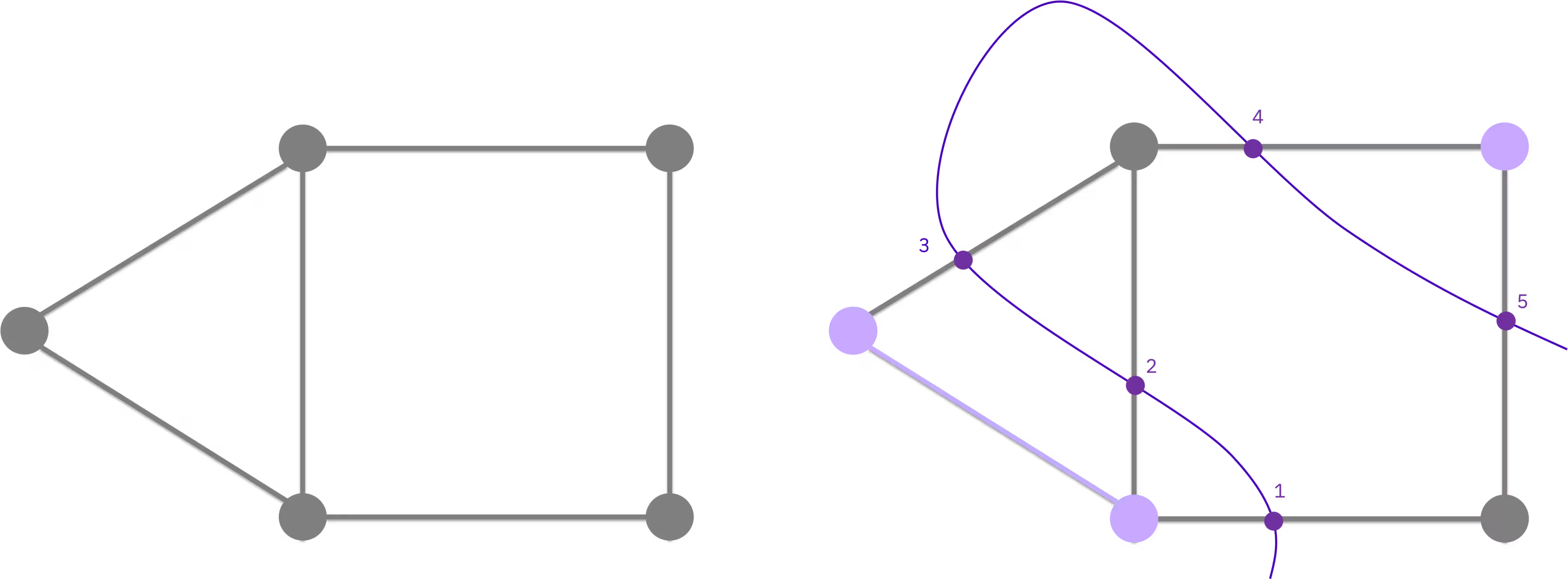
Ang Quantum Approximate Optimization Algorithm (QAOA) ay isang hybrid quantum-classical iterative method para sa paglutas ng combinatorial optimization problems. Sa tutorial na ito, gagamitin mo ang QAOA upang lutasin ang maximum-cut (max-cut) problem — isang NP-hard optimization problem na may mga aplikasyon sa clustering, network science, at statistical physics. Sa isang graph ng mga node na konektado ng mga edge, ang layunin ay hatiin ang mga node sa dalawang set nang sa gayon ang bilang ng mga edge na tumatahak sa partition ay pinakamataas.

Mula sa classical optimization tungo sa quantum circuits

Ang max-cut ay maaaring ipahayag bilang isang classical binary optimization problem. Ang bawat node ay binibigyan ng binary variable na $x_i \in \{0, 1\}$ na nagsasaad kung aling set ito kabilang. Ang layunin ay i-maximize ang bilang ng mga edge kung saan ang mga endpoint ay nasa magkaibang set:

$$\max_{x \in \{0,1\}^n} \sum_{(i,j)} x_i + x_j - 2x_ix_j.$$

Ito ay katumbas ng isang Quadratic Unconstrained Binary Optimization (QUBO) problem na may anyong $\min_x\, x^T Q x$. Sa pamamagitan ng isang karaniwang variable substitution ($x_i \to (1 - Z_i)/2$), ang QUBO ay maaaring isulat muli bilang isang cost Hamiltonian na ang ground state ay naka-encode sa optimal na solusyon. Sa pangkalahatan, ang Hamiltonian na ito ay may parehong quadratic at linear terms:

$$H_C = \sum_{ij} Q_{ij} \, Z_i Z_j + \sum_i b_i \, Z_i.$$

Para sa unweighted max-cut problem na isinasaalang-alang dito, ang linear coefficients ay nawawala ($b_i = 0$) at $Q_{ij} = 1$ para sa bawat edge, kaya naiiwan ang mas simpleng anyong $H_C = \sum_{(i,j) \in E} Z_i Z_j$ na bubuuin mo sa code sa ibaba. Ang mas pangkalahatang anyo sa itaas ang kakailanganin mo upang iakma ang workflow na ito sa weighted graphs o iba pang QUBO-expressible problems.

Paano gumagana ang QAOA

Inihahanda ng QAOA ang mga kandidatong solusyon sa pamamagitan ng pag-apply ng alternating layers ng dalawang operator sa isang initial superposition state na $H^{\otimes n}|0\rangle$: ang cost operator na $e^{-i\gamma_k H_C}$ at isang mixer operator na $e^{-i\beta_k H_m}$. Ang mga angle na $\gamma_k$ at $\beta_k$ ay ino-optimize sa isang classical feedback loop; sinusuri ng quantum computer ang cost function, at ina-update ng isang classical optimizer ang mga parameter hanggang sa convergence. Ang iterative loop na ito ay tumatakbo sa loob ng isang Qiskit Runtime session, na nagpapanatiling naka-reserve ang quantum device sa kabuuan ng mga iteration para sa mas mababang latency.

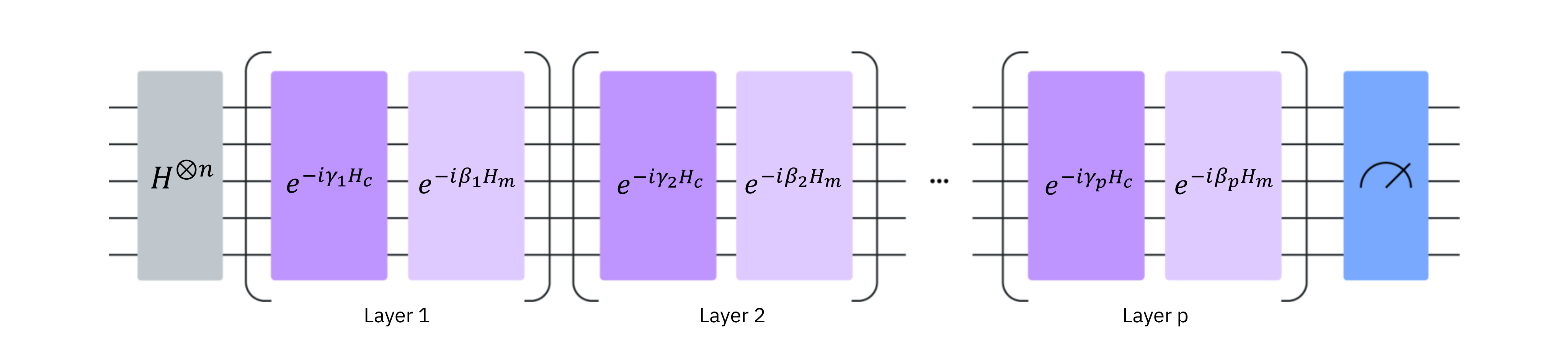
Para sa mas malalim na pagtalakay sa QAOA theory, kasama ang buong QUBO-to-Hamiltonian derivation, tingnan ang QAOA course module.

Sa tutorial na ito, lulutasin mo muna ang max-cut sa isang maliit na five-node graph, pagkatapos ay i-scale ang parehong workflow sa isang 100-node utility-scale problem sa tunay na hardware. Tala sa plan access: Ginagamit ng tutorial na ito ang Qiskit Runtime sessions, na available lamang sa Premium Plan. Kung nasa Open Plan ka, hindi mo mapapatakbo ang tutorial na ito gaya ng nakasulat; sa halip, kailangan mong palitan ang Session ng job mode (ibig sabihin, isumite ang bawat iteration bilang independent job sa halip na ibalot ang optimization loop sa with Session(...)). Tatakbo pa rin ang workflow, ngunit ang bawat iteration ay magdurusa sa buong queue latency sa halip na muling gamitin ang isang naka-reserve na device. Tingnan ang Overview of available plans para sa karagdagang impormasyon.

Mga kinakailangan

Bago magsimula sa tutorial na ito, siguraduhing mayroon kang sumusunod na naka-install:

• Qiskit SDK v2.0 o mas bago, na may visualization support
• Qiskit Runtime v0.22 o mas bago (pip install qiskit-ibm-runtime)

Bilang karagdagan, kakailanganin mo ng access sa isang instance sa IBM Quantum® Platform.

Setup

# Added by doQumentation — required packages for this notebook
!pip install -q matplotlib numpy qiskit qiskit-ibm-runtime rustworkx scipy

import matplotlib.pyplot as plt
import rustworkx as rx
from rustworkx.visualization import mpl_draw as draw_graph
import numpy as np
from scipy.optimize import minimize
from collections import defaultdict
from typing import Sequence

from qiskit.quantum_info import SparsePauliOp
from qiskit.circuit.library import QAOAAnsatz
from qiskit.transpiler.preset_passmanagers import generate_preset_pass_manager

from qiskit_ibm_runtime import QiskitRuntimeService
from qiskit_ibm_runtime import Session, EstimatorV2 as Estimator
from qiskit_ibm_runtime import SamplerV2 as Sampler

Small-scale example

Ang seksyong ito ay dumadaan sa bawat hakbang ng QAOA workflow sa isang maliit na five-node max-cut instance. Sa kabila ng label na "small-scale", ang halimbawang ito ay tumatakbo pa rin sa tunay na IBM Quantum hardware — pumipili ang code ng isang backend na may 127 o higit pang qubits at isinasagawa ang circuit doon. Simulan ang iyong problema sa pamamagitan ng paglikha ng isang graph na may $n=5$ nodes.

n_small = 5

graph = rx.PyGraph()
graph.add_nodes_from(np.arange(0, n_small, 1))
edge_list = [
    (0, 1, 1.0),
    (0, 2, 1.0),
    (0, 4, 1.0),
    (1, 2, 1.0),
    (2, 3, 1.0),
    (3, 4, 1.0),
]
graph.add_edges_from(edge_list)
draw_graph(graph, node_size=600, with_labels=True)

Step 1: Map classical inputs to a quantum problem

I-map ang classical graph sa mga quantum circuits at operators. Tulad ng inilarawan sa Background, para sa unweighted max-cut ang cost Hamiltonian ay bumababa sa $H_C = \sum_{(i,j) \in E} Z_i Z_j$, at gumagamit ang QAOA ng isang parametrized ansatz circuit upang ihanda ang mga kandidatong ground state ng $H_C$.

Buuin ang cost Hamiltonian

I-convert ang mga graph edge sa Pauli $Z_iZ_j$ terms upang buuin ang $H_C$ (tingnan ang Background para sa derivation).

def build_max_cut_paulis(
    graph: rx.PyGraph,
) -> list[tuple[str, list[int], float]]:
    """Convert graph edges to a list of ZZ Pauli terms.

    The returned list is in the sparse format expected by
    ``SparsePauliOp.from_sparse_list``: each element is
    ``(pauli_string, qubit_indices, coefficient)``.
    """
    pauli_list = []
    for edge in list(graph.edge_list()):
        weight = graph.get_edge_data(edge[0], edge[1])
        pauli_list.append(("ZZ", [edge[0], edge[1]], weight))
    return pauli_list

max_cut_paulis = build_max_cut_paulis(graph)
cost_hamiltonian = SparsePauliOp.from_sparse_list(max_cut_paulis, n_small)
print("Cost Function Hamiltonian:", cost_hamiltonian)

Cost Function Hamiltonian: SparsePauliOp(['IIIZZ', 'IIZIZ', 'ZIIIZ', 'IIZZI', 'IZZII', 'ZZIII'],
              coeffs=[1.+0.j, 1.+0.j, 1.+0.j, 1.+0.j, 1.+0.j, 1.+0.j])

Buuin ang QAOA ansatz circuit

Gamitin ang QAOAAnsatz upang buuin ang parametrized QAOA circuit mula sa cost Hamiltonian. Dito gumagamit tayo ng reps=2 (dalawang QAOA layers, apat na parameter: $\beta_0, \beta_1, \gamma_0, \gamma_1$).

circuit = QAOAAnsatz(cost_operator=cost_hamiltonian, reps=2)
circuit.measure_all()

circuit.draw("mpl")

circuit.parameters

ParameterView([ParameterVectorElement(β[0]), ParameterVectorElement(β[1]), ParameterVectorElement(γ[0]), ParameterVectorElement(γ[1])])

Step 2: Optimize problem for quantum hardware execution

I-transpile ang abstract circuit sa hardware-native instructions. Hinahawakan ng hakbang na ito ang qubit mapping, gate decomposition, routing, at error suppression. Tingnan ang transpilation documentation para sa karagdagang impormasyon.

service = QiskitRuntimeService()
backend = service.least_busy(
    operational=True, simulator=False, min_num_qubits=127
)
print(backend)

# Create pass manager for transpilation. Level 3 is the most aggressive
# preset: slower to transpile, but produces shorter circuits that are
# more robust to hardware noise.
pm = generate_preset_pass_manager(optimization_level=3, backend=backend)

candidate_circuit = pm.run(circuit)
candidate_circuit.draw("mpl", fold=False, idle_wires=False)

<IBMBackend('ibm_pittsburgh')>

Step 3: Execute using Qiskit primitives

Ang QAOA optimization loop ay tumatakbo sa loob ng isang Qiskit Runtime session upang panatilihing naka-reserve ang device sa kabuuan ng mga iteration. Sinusuri ng isang Estimator ang $\langle H_C \rangle$ sa bawat hakbang, at ina-update ng isang classical optimizer (COBYLA) ang mga parameter hanggang sa convergence.

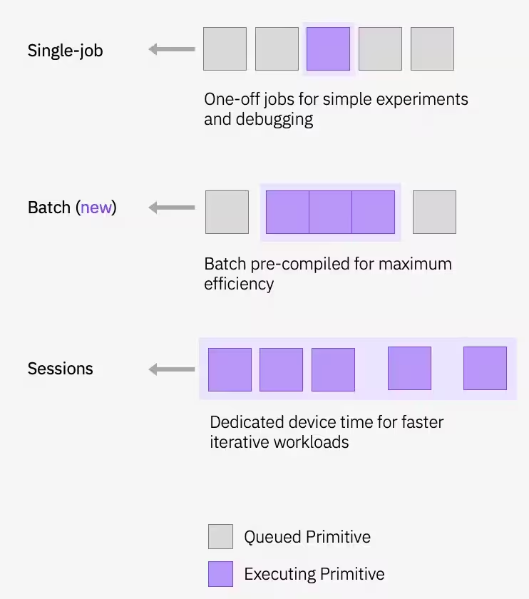I-define ang mga initial parameter at patakbuhin ang optimization loop:

# QAOA doesn't prescribe principled default angles — any bounded choice
# works as a warm start for problems this small. beta and gamma are
# periodic (beta in [0, pi] and gamma in [0, 2*pi] modulo the underlying
# Pauli-rotation periods), and pi/2 and pi are just midpoints of those
# ranges. For harder problems you would typically warm start from known
# good angles or transfer parameters from smaller instances.
initial_gamma = np.pi
initial_beta = np.pi / 2
init_params = [initial_beta, initial_beta, initial_gamma, initial_gamma]

def cost_func_estimator(params, ansatz, hamiltonian, estimator):
    # transform the observable defined on virtual qubits to
    # an observable defined on all physical qubits
    isa_hamiltonian = hamiltonian.apply_layout(ansatz.layout)

    pub = (ansatz, isa_hamiltonian, params)
    job = estimator.run([pub])

    results = job.result()[0]
    cost = results.data.evs

    objective_func_vals.append(cost)

    return cost

objective_func_vals = []  # Global variable
with Session(backend=backend) as session:
    # If using qiskit-ibm-runtime<0.24.0, change `mode=` to `session=`
    estimator = Estimator(mode=session)
    estimator.options.default_shots = 1000

    # Set simple error suppression/mitigation options
    estimator.options.dynamical_decoupling.enable = True
    estimator.options.dynamical_decoupling.sequence_type = "XY4"
    estimator.options.twirling.enable_gates = True
    estimator.options.twirling.num_randomizations = "auto"
    estimator.options.environment.job_tags = ["TUT_QAOA"]

    result = minimize(
        cost_func_estimator,
        init_params,
        args=(candidate_circuit, cost_hamiltonian, estimator),
        method="COBYLA",
        tol=1e-2,
    )
    print(result)

message: Return from COBYLA because the trust region radius reaches its lower bound.
 success: True
  status: 0
     fun: -2.0402211719947774
       x: [ 3.041e+00  1.212e+00  2.081e+00  4.471e+00]
    nfev: 36
   maxcv: 0.0

Nagawa ng optimizer na bawasan ang cost at makahanap ng mas mahusay na parameter para sa circuit.

Ang isang maayos na bumababang curve na pumapatag ang signature ng convergence. Ang isang maingay, non-monotonic na curve ay karaniwang nagpapahiwatig na may kailangang pansinin sa upstream; ang mga karaniwang sanhi ay masyadong kaunting shots bawat evaluation (mataas na estimator variance), mahinang initial parameters, o isang circuit na ang depth ay dinodominahan ng hardware noise. Ang COBYLA ay derivative-free at medyo matatag sa katamtamang noise, ngunit kapag inaapakan ng noise ang aktuwal na cost improvements bawat hakbang, hindi na masabi ng linear-approximation model nito ang tunay na descent mula sa random jitter at naglilibot ang optimizer.

plt.figure(figsize=(12, 6))
plt.plot(objective_func_vals)
plt.xlabel("Iteration")
plt.ylabel("Cost")
plt.show()

I-assign ang mga naka-optimize na parameter at i-sample ang final distribution gamit ang Sampler primitive.

optimized_circuit = candidate_circuit.assign_parameters(result.x)
optimized_circuit.draw("mpl", fold=False, idle_wires=False)

# If using qiskit-ibm-runtime<0.24.0, change `mode=` to `backend=`
sampler = Sampler(mode=backend)
sampler.options.default_shots = 10000

# Set simple error suppression/mitigation options
sampler.options.dynamical_decoupling.enable = True
sampler.options.dynamical_decoupling.sequence_type = "XY4"
sampler.options.twirling.enable_gates = True
sampler.options.twirling.num_randomizations = "auto"

sampler.options.environment.job_tags = ["TUT_QAOA"]

pub = (optimized_circuit,)
job = sampler.run([pub], shots=int(1e4))
counts_int = job.result()[0].data.meas.get_int_counts()
counts_bin = job.result()[0].data.meas.get_counts()
shots = sum(counts_int.values())
final_distribution_int = {key: val / shots for key, val in counts_int.items()}
final_distribution_bin = {key: val / shots for key, val in counts_bin.items()}
print(final_distribution_int)

{18: 0.039, 5: 0.0665, 20: 0.0973, 29: 0.0063, 9: 0.0899, 13: 0.0379, 2: 0.0047, 1: 0.0153, 11: 0.0932, 14: 0.0327, 12: 0.0314, 25: 0.0193, 21: 0.0398, 6: 0.0224, 4: 0.0197, 10: 0.0387, 3: 0.0181, 26: 0.07, 17: 0.0327, 19: 0.0332, 22: 0.0914, 24: 0.007, 0: 0.0033, 8: 0.0066, 30: 0.0158, 28: 0.0169, 27: 0.0222, 16: 0.0073, 7: 0.0057, 23: 0.0062, 15: 0.0054, 31: 0.0041}

Step 4: Post-process and return result in desired classical format

Kunin ang pinaka-malamang na bitstring mula sa sampled distribution. Kumakatawan ito sa pinakamahusay na cut na natagpuan ng QAOA.

# auxiliary functions to sample most likely bitstring
def to_bitstring(integer, num_bits):
    result = np.binary_repr(integer, width=num_bits)
    return [int(digit) for digit in result]

keys = list(final_distribution_int.keys())
values = list(final_distribution_int.values())
most_likely = keys[np.argmax(np.abs(values))]
most_likely_bitstring = to_bitstring(most_likely, len(graph))
most_likely_bitstring.reverse()

print("Result bitstring:", most_likely_bitstring)

Result bitstring: [0, 0, 1, 0, 1]

plt.rcParams.update({"font.size": 10})
final_bits = final_distribution_bin
values = np.abs(list(final_bits.values()))
top_4_values = sorted(values, reverse=True)[:4]
positions = []
for value in top_4_values:
    positions.append(np.where(values == value)[0])
fig = plt.figure(figsize=(11, 6))
ax = fig.add_subplot(1, 1, 1)
plt.xticks(rotation=45)
plt.title("Result Distribution")
plt.xlabel("Bitstrings (reversed)")
plt.ylabel("Probability")
ax.bar(list(final_bits.keys()), list(final_bits.values()), color="tab:grey")
for p in positions:
    ax.get_children()[int(p[0])].set_color("tab:purple")
plt.show()

I-visualize ang pinakamahusay na cut

Mula sa optimal bitstring, maaari mong i-visualize ang cut na ito sa orihinal na graph.

# auxiliary function to plot graphs
def plot_result(G, x):
    colors = ["tab:grey" if i == 0 else "tab:purple" for i in x]
    pos, _default_axes = rx.spring_layout(G), plt.axes(frameon=True)
    rx.visualization.mpl_draw(
        G, node_color=colors, node_size=100, alpha=0.8, pos=pos
    )

plot_result(graph, most_likely_bitstring)

Ngayon, kalkulahin ang halaga ng cut:

def evaluate_sample(x: Sequence[int], graph: rx.PyGraph) -> float:
    assert len(x) == len(
        list(graph.nodes())
    ), "The length of x must coincide with the number of nodes in the graph."
    return sum(
        x[u] * (1 - x[v]) + x[v] * (1 - x[u])
        for u, v in list(graph.edge_list())
    )

cut_value = evaluate_sample(most_likely_bitstring, graph)
print("The value of the cut is:", cut_value)

The value of the cut is: 5

Para sa isang graph na ganito kaliit, madaling i-brute-force ang tunay na optimum, kaya maaari mong i-double-check ang mga resulta sa pamamagitan ng paghahambing ng QAOA result laban sa eksaktong sagot.

# Classical baseline: enumerate all 2**n_small bitstrings and take the best cut.
def brute_force_max_cut(graph: rx.PyGraph) -> tuple[int, list[int]]:
    n = len(list(graph.nodes()))
    best_cut = -1
    best_x: list[int] = []
    for i in range(2**n):
        x = [(i >> k) & 1 for k in range(n)]
        cut = evaluate_sample(x, graph)
        if cut > best_cut:
            best_cut = int(cut)
            best_x = x
    return best_cut, best_x

classical_best, classical_x = brute_force_max_cut(graph)
print(f"Classical optimum (brute force): {classical_best}")
print(f"QAOA cut value:                  {cut_value}")

Classical optimum (brute force): 5
QAOA cut value:                  5

Large-scale hardware example

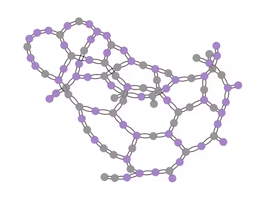
May access ka sa maraming device na may higit sa 100 qubits sa IBM Quantum Platform. Pumili ng isa kung saan lulutasin ang max-cut sa isang 100-node weighted graph. Ito ay isang "utility-scale" problem. Sinusunod ng workflow ang parehong mga hakbang gaya ng sa itaas, na inilapat sa isang mas malaking graph.

End-to-end workflow sa utility scale

Ang lahat ng apat na hakbang ay ipinapakita sa ibaba, na inilapat sa 100-node graph. Ang istruktura ay pareho sa small-scale walkthrough: map, transpile, execute, post-process — ngunit may mas malaking problema at hinati sa apat na cell sa ibaba para sa kalinawan.

# Precomputed parity lookup table: _PARITY[b] = +1 if popcount(b) is even, else -1.
# We use this to vectorize expectation-value evaluation across all Pauli terms.
_PARITY = np.array(
    [-1 if bin(i).count("1") % 2 else 1 for i in range(256)],
    dtype=np.complex128,
)

def evaluate_sparse_pauli(state: int, observable: SparsePauliOp) -> complex:
    """Expectation value of a SparsePauliOp on a single computational-basis state.

    For a Z-only observable (which QAOA cost Hamiltonians are, after the
    QUBO-to-Hamiltonian mapping), the eigenvalue of each Pauli term on a
    computational-basis state is simply (-1)**popcount(z_mask AND state),
    i.e., the parity of the bitwise-AND of the term's Z-support and the
    measured bitstring.

    This routine packs the Z-support of every Pauli term into bytes, ANDs
    them against the measured state in a single vectorized op, and looks up
    the parity in _PARITY. For a 100-qubit / ~hundreds-of-terms Hamiltonian
    over 10_000 samples, this is dramatically faster than calling
    SparsePauliOp.expectation_value per sample.
    """
    packed_uint8 = np.packbits(observable.paulis.z, axis=1, bitorder="little")
    state_bytes = np.frombuffer(
        state.to_bytes(packed_uint8.shape[1], "little"), dtype=np.uint8
    )
    reduced = np.bitwise_xor.reduce(packed_uint8 & state_bytes, axis=1)
    return np.sum(observable.coeffs * _PARITY[reduced])

def best_solution(samples, hamiltonian):
    """Return the sampled bitstring (as int) with the lowest Hamiltonian cost."""
    min_cost = float("inf")
    min_sol = None
    for bit_str in samples.keys():
        candidate_sol = int(bit_str)
        fval = evaluate_sparse_pauli(candidate_sol, hamiltonian).real
        if fval <= min_cost:
            min_cost = fval
            min_sol = candidate_sol
    return min_sol

def _plot_cdf(objective_values: dict, ax, color):
    x_vals = sorted(objective_values.keys(), reverse=True)
    y_vals = np.cumsum([objective_values[x] for x in x_vals])
    ax.plot(x_vals, y_vals, color=color)

def plot_cdf(dist, ax, title):
    _plot_cdf(dist, ax, "C1")
    ax.vlines(min(list(dist.keys())), 0, 1, "C1", linestyle="--")
    ax.set_title(title)
    ax.set_xlabel("Objective function value")
    ax.set_ylabel("Cumulative distribution function")
    ax.grid(alpha=0.3)

def samples_to_objective_values(samples, hamiltonian):
    """Convert the samples to values of the objective function."""
    objective_values = defaultdict(float)
    for bit_str, prob in samples.items():
        candidate_sol = int(bit_str)
        fval = evaluate_sparse_pauli(candidate_sol, hamiltonian).real
        objective_values[fval] += prob
    return objective_values

Step 1: Buuin ang graph, cost Hamiltonian, at ansatz.

# Step 1: build the 100-node graph, cost Hamiltonian, and QAOA ansatz.
n_large = 100
graph_100 = rx.PyGraph()
graph_100.add_nodes_from(np.arange(0, n_large, 1))
elist = []
for edge in backend.coupling_map:
    if edge[0] < n_large and edge[1] < n_large:
        elist.append((edge[0], edge[1], 1.0))
graph_100.add_edges_from(elist)

max_cut_paulis_100 = build_max_cut_paulis(graph_100)
cost_hamiltonian_100 = SparsePauliOp.from_sparse_list(
    max_cut_paulis_100, n_large
)

circuit_100 = QAOAAnsatz(cost_operator=cost_hamiltonian_100, reps=1)
circuit_100.measure_all()

Step 2: I-transpile para sa napiling hardware backend.

# Step 2: transpile for hardware.
pm = generate_preset_pass_manager(optimization_level=3, backend=backend)
candidate_circuit_100 = pm.run(circuit_100)

Step 3: Patakbuhin ang QAOA optimization loop sa loob ng isang session, pagkatapos ay mag-sample.

# Step 3: run the QAOA optimization loop on the device, then sample the
# final distribution with the optimized parameters.
initial_gamma = np.pi
initial_beta = np.pi / 2
init_params = [initial_beta, initial_gamma]

objective_func_vals = []  # Global variable
with Session(backend=backend) as session:
    estimator = Estimator(mode=session)
    estimator.options.default_shots = 1000

    # Set simple error suppression/mitigation options
    estimator.options.dynamical_decoupling.enable = True
    estimator.options.dynamical_decoupling.sequence_type = "XY4"
    estimator.options.twirling.enable_gates = True
    estimator.options.twirling.num_randomizations = "auto"
    estimator.options.environment.job_tags = ["TUT_QAOA"]

    result = minimize(
        cost_func_estimator,
        init_params,
        args=(candidate_circuit_100, cost_hamiltonian_100, estimator),
        method="COBYLA",
    )
    print(result)

# Assign optimal parameters and sample the final distribution.
optimized_circuit_100 = candidate_circuit_100.assign_parameters(result.x)

sampler = Sampler(mode=backend)
sampler.options.default_shots = 10000

# Set simple error suppression/mitigation options
sampler.options.dynamical_decoupling.enable = True
sampler.options.dynamical_decoupling.sequence_type = "XY4"
sampler.options.twirling.enable_gates = True
sampler.options.twirling.num_randomizations = "auto"

# Add a unique tag to the job execution
sampler.options.environment.job_tags = ["TUT_QAOA"]

pub = (optimized_circuit_100,)
job = sampler.run([pub], shots=int(1e4))

counts_int = job.result()[0].data.meas.get_int_counts()
shots = sum(counts_int.values())
final_distribution_100_int = {
    key: val / shots for key, val in counts_int.items()
}

message: Return from COBYLA because the trust region radius reaches its lower bound.
 success: True
  status: 0
     fun: -17.172689238986344
       x: [ 2.574e+00  4.166e+00]
    nfev: 28
   maxcv: 0.0

Step 4: I-post-process ang sampled distribution upang kunin ang pinakamahusay na cut.

# Step 4: find the best-cost sample and evaluate its cut value.
best_sol_100 = best_solution(final_distribution_100_int, cost_hamiltonian_100)
best_sol_bitstring_100 = to_bitstring(int(best_sol_100), len(graph_100))
best_sol_bitstring_100.reverse()

print("Result bitstring:", best_sol_bitstring_100)

cut_value_100 = evaluate_sample(best_sol_bitstring_100, graph_100)
print("The value of the cut is:", cut_value_100)

Result bitstring: [1, 1, 0, 1, 1, 0, 1, 1, 1, 0, 1, 0, 1, 1, 1, 0, 1, 1, 1, 1, 0, 0, 1, 0, 0, 1, 1, 0, 1, 0, 1, 0, 1, 1, 0, 1, 1, 0, 0, 0, 0, 0, 1, 1, 0, 1, 0, 0, 0, 1, 0, 0, 1, 0, 1, 0, 0, 1, 1, 1, 1, 1, 0, 1, 0, 1, 0, 0, 0, 1, 0, 1, 0, 1, 0, 0, 0, 0, 1, 0, 0, 1, 0, 1, 1, 1, 1, 0, 1, 0, 1, 0, 1, 1, 1, 0, 1, 1, 1, 0]
The value of the cut is: 156

Suriin na ang cost na minimize sa optimization loop ay nag-converge, at i-visualize ang mga resulta.

# Plot convergence
plt.figure(figsize=(12, 6))
plt.plot(objective_func_vals)
plt.xlabel("Iteration")
plt.ylabel("Cost")
plt.show()

# Visualize the cut
plot_result(graph_100, best_sol_bitstring_100)

# Plot cumulative distribution function
result_dist = samples_to_objective_values(
    final_distribution_100_int, cost_hamiltonian_100
)
fig, ax = plt.subplots(1, 1, figsize=(8, 6))
plot_cdf(result_dist, ax, backend.name)

Mga susunod na hakbang

Kung nakita mong kawili-wili ang gawaing ito, maaaring interesado ka sa sumusunod na materyal:

Mga rekomendasyon

• Advanced techniques for QAOA — tinatalakay ang mga advanced na estratehiya para sa pagpapabuti ng QAOA performance
• Multi-objective optimization challenge — subukin ang iyong mga kasanayan sa community challenge na ito sa multi-objective quantum optimization
• Transpilation documentation para sa fine-tuning ng circuit optimization
• Error suppression and mitigation para sa pagpapabuti ng hardware results