Low-overhead error detection na may spacetime codes

Usage estimate: 4 minuto sa isang Heron processor (ibm_kingston o katumbas) (TANDAAN: Ito ay tantiya lamang. Maaaring mag-iba ang iyong runtime.)

Mga learning outcome

• Kung paano nakakatuklas ang spacetime Pauli checks ng logical errors sa Clifford circuits, at kung paano pinapataas ng postselecting sa mga syndrome nito ang fidelity ng isang sampled distribution.

• Kung paano gamitin ang qiskit-paulice package upang hanapin at ipasok ang hardware-efficient checks nang awtomatiko gamit ang get_check_qubits, NoiseModel, at add_pauli_checks.

• Kung paano tantiyahin ang fidelity ng isang stabilizer state sa pamamagitan ng pag-sample ng mga stabilizer nito at postselecting sa check syndromes.

• Kung paano patakbuhin ang buong error-detection workflow sa IBM Quantum® hardware at ikumpara ang noisy at postselected fidelities.

Prerequisites

• Mga batayan ng hardware para sa utility-scale quantum computing.

• Ang Clifford at stabilizer formalism, kasama ang kung paano inilalarawan ng stabilizer group ang isang purong stabilizer state.

Background

Ang Low-overhead error detection with spacetime codes [1] nina Simon Martiel at Ali Javadi-Abhari ay nagpapakilala ng isang method para sa pagtukoy ng logical errors sa Clifford-dominated circuits na nasa pagitan ng buong error correction at mas magaan na error mitigation. Ang ideya ay binuo sa coherent Pauli checks (CPC) mula sa Single-shot error mitigation by coherent Pauli checks [2] nina van den Berg at iba pa. Sa parehong approach, ang isang Clifford na "payload" circuit ay entangled sa mga ancilla qubits upang suriin ang ilang invariant. Ang pagsukat sa mga ancilla ay bumubuo ng isang syndrome na nag-uulat kung may nadetektang error sa panahon ng execution. Ang pagpanatili lamang ng mga sample na walang nadetektang error ay nagpapabuti sa fidelity ng sampled distribution, sa gastos ng pababang postselection rate.

Ang pangunahing pagkakaiba sa pagitan ng coherent Pauli checks at spacetime checks ay ang mga operator na sinusukat nila. Ang coherent Pauli checks ay sumusukat ng time-localized, high-weight operators. Sa mga qubit topologies na may limitadong connectivity, tulad ng heavy hex, ang mga check na iyon ay nangangailangan ng maraming SWAP gates at kadalasang ginagawang masyadong malalim ang circuit upang maging praktikal. Sa halip, ang pagpapatupad ng mga check bilang spacetime codes ay nagbabahagi ng bawat check sa buong payload circuit sa espasyo at oras. Nagbubunga ito ng hardware-efficient encoding na nananatiling epektibo sa pagtukoy ng logical errors habang pinapanatiling mababa ang qubit at depth overhead.

Ano ang ginagawa ng qiskit-paulice package

Ino-automate ng qiskit-paulice package ang pagbuo ng mga check na ito upang hindi mo na kailangang buuin ang mga ito nang manu-mano. Ang pangunahing tungkulin nito ay hanapin at ipasok ang mga valid na spacetime Pauli checks sa mga lokasyon sa isang circuit na nag-maximize ng error detection habang minimize ang qubit overhead. Ang isang check ay valid kapag ang mga operator nito ay hindi nagbabago sa logical action ng payload circuit, low-weight kapag gumagamit ito ng kaunting entangling gates, at effective kapag natutukoy nito ang malaking bahagi ng mga error, kaugnay ng noise na dala mismo ng check. Sini-score ng package ang mga kandidatong check laban sa isang noise model at kinokomit ang pinakamahusay sa circuit. Gumagamit ang tutorial na ito ng tatlong API method:

• Sinusuri ng get_check_qubits ang coupling map ng isang backend at nagbabalik ng mga target at ancilla qubit pairs. Ang isang check sa target_qubits[i] ay gumagamit ng ancilla_qubits[i].

• Bumubuo ang NoiseModel.from_backend ng magaspang na noise model mula sa backend benchmark data. Sini-score ng modelo ang mga kandidatong check, kaya hindi kinakailangan ang eksakto, learned na noise model. Para sa isang learned Pauli-Lindblad model, tingnan ang NoiseModel.from_pauli_lindblad_maps.

• Naghahanap at nagpapasok ang add_pauli_checks ng mga check sa isang circuit. Nagbabalik ito ng sequence ng CheckedCircuit objects na may dumaraming bilang ng checks, at ang bawat object ay nagbibigay ng get_postselection_method na nagma-map ng isang sinukat na bitstring sa isang syndrome vector. Pinipili ng argument na cost ang function na sumusukat ng isang check (gamma, ang sampling overhead ng postselected inverse noise channel, o LER, ang logical error rate). Pinipili ng argument na method ang search strategy (windowed, genetic, o windowed_genetic). Ginagamit ng tutorial na ito ang cost="gamma" at method="windowed", na magkasamang nagbibigay ng deterministic, reproducible na pagpili ng check.

Tantiyahin ang fidelity mula sa stabilizer sampling

Upang sukatin kung gaano kahusay gumagana ang error detection, maaari mong tantiyahin ang fidelity ng stabilizer state na $|\psi\rangle = U|0\rangle^{\otimes n}$ na ideal na inihahanda ng circuit laban sa noisy state na $\rho$ na aktwal na inilalabas ng hardware. Ang projector sa isang purong stabilizer state na $|\psi\rangle$ ay katumbas ng uniform na average sa $2^n$ elements ng stabilizer group nito na $\mathcal{S}$:

$|\psi\rangle\langle\psi| = \frac{1}{2^n}\sum_{G \in \mathcal{S}} G.$

Ang pagpapalit nito sa fidelity ay nagbibigay ng fidelity ng $\rho$ bilang average expectation value ng bawat stabilizer na $G \in \mathcal{S}$ kaugnay ng $\rho$:

$F = \mathrm{Tr}(\rho|\psi\rangle\langle\psi|) = \frac{1}{2^n} \sum_{G \in \mathcal{S}} \mathrm{Tr}(\rho G) = \frac{1}{2^n} \sum_{G \in \mathcal{S}} \langle G \rangle_\rho.$

Para sa mas malalaking problema, hindi praktikal ang pag-enumerate ng lahat ng $2^n$ stabilizers, kaya maaari mong tantiyahin ang fidelity mula sa isang random sample. Ang pagkuha ng $M$ stabilizers na $G_1, \ldots, G_M$ nang uniform na random mula sa $\mathcal{S}$ ay nagbibigay ng isang unbiased na tantiya:

$\hat F_M = \frac{1}{M} \sum_{i=1}^M \langle G_i \rangle_\rho.$

Dahil ang isang Clifford circuit ay naghahanda ng isang stabilizer state, maaari mong tantiyahin ang fidelity nito nang direkta mula sa sampled expectation values ng mga stabilizer nito. Sasabayan muna ng tutorial na ito ang workflow sa isang simulator gamit ang maliit na circuit, pagkatapos ay patatakbuhin ang parehong workflow sa hardware gamit ang mas malaki at mas malalim na circuit. Habang naglalaman ang mga circuit ng mas maraming non-Clifford operations, mabilis na bumababa ang bilang ng mga valid na check, kaya ang method ay mas epektibo para sa mga Clifford-dominated na circuit.

Requirements

Bago simulan ang tutorial na ito, siguraduhing na-install mo na ang mga sumusunod:

• Qiskit SDK v2.0 o mas bago, na may suportang visualization

• Qiskit Runtime v0.40 o mas bago (pip install qiskit-ibm-runtime)

• Qiskit Aer v0.17 o mas bago (pip install qiskit-aer)

• Qiskit Paulice (pip install qiskit-paulice)

• tqdm (pip install tqdm)

Setup

I-import ang mga kinakailangang library at tukuyin ang mga helper function na hindi available bilang import. Ang random_clifford_circuit function ay bumubuo ng brickwork random Clifford payload, ang find_check_layout ay naghahanap sa coupling map ng isang backend ng low-error qubit path na may maraming available na ancilla, ang learned_noise_model ay ginagawang qiskit-paulice noise model ang output ng NoiseLearner, ang append_basis_rotation ay umiikot sa isang circuit upang masukat ang isang stabilizer sa computational basis, ang expectation ay kumukuwenta ng stabilizer expectation value mula sa mga sampled count, at ang cum_mean_sem ay sumusubaybay sa running fidelity estimate.

# Added by doQumentation — required packages for this notebook
!pip install -q matplotlib numpy qiskit qiskit-aer qiskit-ibm-runtime qiskit-paulice tqdm

# Standard library imports
import random
import time

# External libraries
import matplotlib.pyplot as plt
import numpy as np
from tqdm import tqdm

# Qiskit
from qiskit import QuantumCircuit
from qiskit.quantum_info import Clifford, Pauli, PauliLindbladMap, PauliList
from qiskit.result import sampled_expectation_value
from qiskit.transpiler import generate_preset_pass_manager
from qiskit.visualization import plot_coupling_map

# Qiskit Aer
from qiskit_aer import AerSimulator
from qiskit_aer.noise import NoiseModel as AerNoiseModel
from qiskit_aer.noise import ReadoutError, depolarizing_error

# Qiskit IBM Runtime
from qiskit_ibm_runtime import NoiseLearner, QiskitRuntimeService
from qiskit_ibm_runtime import SamplerV2 as Sampler

# Qiskit Paulice
from qiskit_paulice import add_pauli_checks
from qiskit_paulice.layout import get_check_qubits
from qiskit_paulice.noise_models import NoiseModel

def random_clifford_circuit(
    num_qubits: int, depth: int, rng: np.random.Generator
) -> QuantumCircuit:
    """Brickwork random Clifford on `num_qubits`, with `depth` CZ layers."""
    qc = QuantumCircuit(num_qubits)
    qc.h(range(num_qubits))
    for d in range(depth):
        for i in range(d % 2, num_qubits - 1, 2):
            qc.cz(i, i + 1)
        for q in range(num_qubits):
            if rng.integers(0, 2):
                qc.sx(q)
            if rng.integers(0, 2):
                qc.s(q)
            if rng.integers(0, 2):
                qc.sx(q)
    return qc

def find_check_layout(
    backend,
    num_qubits: int,
    rng: np.random.Generator,
    num_trials: int = 200,
    max_gate_error: float = 0.03,
    max_readout_error: float = 0.2,
) -> list[int]:
    """Find a low-error path of `num_qubits` qubits with many available ancillas.

    Builds random self-avoiding walks on the coupling map, excluding the qubits
    and two-qubit gates whose reported errors exceed the thresholds, and keeps
    the path that offers the most target and ancilla pairs. Ties are broken by
    the lower average two-qubit gate error along the path.
    """
    target = backend.target
    gate_2q = next(
        name for name in ("cz", "ecr", "cx") if name in target.operation_names
    )

    # Collect per-edge gate errors and per-qubit readout errors
    edge_error = {}
    for qubits, props in target[gate_2q].items():
        edge = tuple(sorted(qubits))
        if props is not None and props.error is not None:
            edge_error[edge] = min(edge_error.get(edge, 1.0), props.error)
    readout_error = {
        qubit: target["measure"][(qubit,)].error
        for (qubit,) in target["measure"]
    }

    # Keep only the edges whose gate and readout errors are acceptable
    adjacency = {}
    for (q1, q2), error in edge_error.items():
        if (
            error <= max_gate_error
            and readout_error.get(q1, 1.0) <= max_readout_error
            and readout_error.get(q2, 1.0) <= max_readout_error
        ):
            adjacency.setdefault(q1, set()).add(q2)
            adjacency.setdefault(q2, set()).add(q1)

    # Random self-avoiding walks; keep the path with the most check pairs
    starts = sorted(adjacency)
    best_path = None
    best_score = (-1, float("inf"))
    for _ in range(num_trials):
        path = [starts[rng.integers(len(starts))]]
        while len(path) < num_qubits:
            options = sorted(adjacency[path[-1]] - set(path))
            if not options:
                break
            path.append(options[rng.integers(len(options))])
        if len(path) < num_qubits:
            continue
        num_pairs = len(get_check_qubits(backend.coupling_map, path)[0])
        mean_error = float(
            np.mean(
                [edge_error[tuple(sorted(e))] for e in zip(path, path[1:])]
            )
        )
        if num_pairs > best_score[0] or (
            num_pairs == best_score[0] and mean_error < best_score[1]
        ):
            best_path, best_score = path, (num_pairs, mean_error)

    if best_path is None:
        raise RuntimeError(
            "No connected low-error path found. Relax the error thresholds."
        )
    return best_path

def learned_noise_model(layer_errors, layout: list[int]) -> NoiseModel:
    """Build a `NoiseModel` from `NoiseLearner` results.

    `NoiseLearner` reports one `PauliLindbladError` per entangling layer, whose
    generators are indexed against that layer's own physical qubits, while
    `NoiseModel.from_pauli_lindblad_maps` expects `PauliLindbladMap`s indexed the
    way `NoiseModel.from_backend` indexes them: by position in `layout`. This
    translates between the two and drops generators that fall outside `layout`.
    """
    phys_to_virt = {phys: virt for virt, phys in enumerate(layout)}
    maps = []
    for layer in layer_errors:
        if layer.error is None:
            continue
        terms = []
        for pauli, rate in zip(
            layer.error.generators, layer.error.rates, strict=True
        ):
            label, indices = [], []
            for local, phys in enumerate(layer.qubits):
                x, z = bool(pauli.x[local]), bool(pauli.z[local])
                if not (x or z):
                    continue
                if phys not in phys_to_virt:
                    break  # generator reaches outside the layout, so skip it
                label.append("Y" if x and z else "X" if x else "Z")
                indices.append(phys_to_virt[phys])
            else:
                if label:
                    terms.append(
                        ("".join(label), tuple(indices), float(rate))
                    )
        # Each map needs a 2-qubit generator to define an entangling layer
        if any(len(t[1]) == 2 for t in terms):
            maps.append(
                PauliLindbladMap.from_sparse_list(
                    terms, num_qubits=len(layout)
                )
            )
    if not maps:
        raise RuntimeError(
            "No usable layer errors. Check that the learner ran on this layout."
        )
    return NoiseModel.from_pauli_lindblad_maps(maps)

def append_basis_rotation(
    circuit: QuantumCircuit, pauli: Pauli
) -> QuantumCircuit:
    """Strip measurements, append basis rotations for `pauli`, and re-measure."""
    out = circuit.remove_final_measurements(inplace=False)
    for q in range(pauli.num_qubits):
        if pauli.x[q]:
            if pauli.z[q]:
                out.sdg(q)
            out.h(q)
    out.measure_all()
    return out

def expectation(counts: dict, pauli: Pauli) -> float:
    """Expectation value of `pauli` from counts measured in the Z basis.

    Pads with identity on any qubits beyond the support of `pauli`, such as the
    check ancillas that appear in the postselected counts.
    """
    if not counts:
        return float("nan")
    n = pauli.num_qubits
    sign = -1 if int(pauli.phase) % 4 == 2 else 1
    total = len(next(iter(counts)))
    label = "".join(
        "Z" if q < n and (pauli.x[q] or pauli.z[q]) else "I"
        for q in range(total - 1, -1, -1)
    )
    return sign * sampled_expectation_value(counts, label)

def cum_mean_sem(values: np.ndarray):
    """Cumulative mean and standard error of the mean, ignoring NaNs."""
    valid = ~np.isnan(values)
    total = np.cumsum(np.where(valid, values, 0.0))
    total_sq = np.cumsum(np.where(valid, values**2, 0.0))
    count = np.maximum(np.cumsum(valid).astype(float), 1)
    mean = total / count
    sem = np.sqrt(np.maximum(total_sq / count - mean**2, 0) / count)
    return np.where(np.cumsum(valid) > 0, mean, np.nan), sem

Halimbawa ng simulator sa maliit na sukat

Tinatalakay ng seksyong ito ang buong workflow sa isang maingay (noisy) na simulator. Gumagamit ito ng backend benchmark data para pumili ng qubit layout at noise model, awtomatikong naghahanap ng mga check, at gumagamit ng postselection sa sampled distribution para ipakita ang pagbuti sa fidelity.

Step 1: I-map ang mga classical input sa isang quantum problem

Ang payload circuit ay isang mababaw (shallow), one-dimensional na brickwork random Clifford circuit. Dahil Clifford ang circuit, naghahanda ito ng stabilizer state na maaari mong tantiyahin ang fidelity nito nang direkta mula sa sampled stabilizer expectation values. Magsimula sa isang mababaw na circuit para madaling i-visualize ang mga check sa susunod na hakbang.

num_qubits = 12
depth = 4
seed = 1764
rng = np.random.default_rng(seed)
np.random.seed(seed)

circuit = random_clifford_circuit(num_qubits, depth, rng)
circuit.measure_all()
circuit.draw("mpl", fold=-1, scale=0.6)

Step 2: I-optimize para sa pagpapatakbo sa quantum hardware

Ang pag-map ng circuit patungo sa hardware ay nagtatakda ng physical qubit layout, ng noise model na nagra-rate sa mga kandidatong check, at ng mga check mismo.

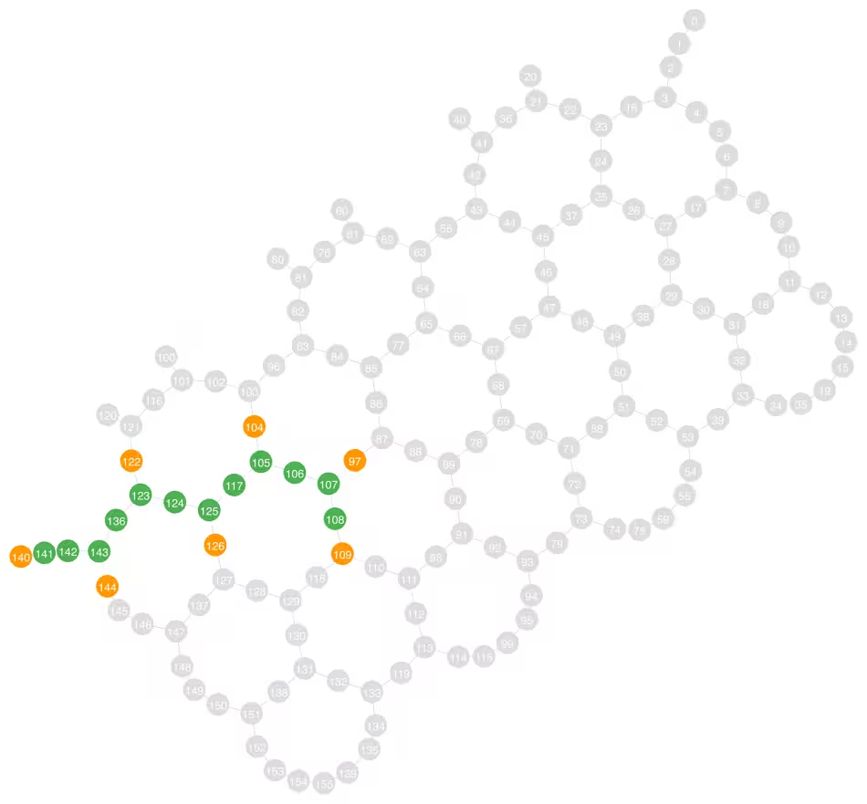
Una, pumili ng backend at hanapin sa coupling map nito ang isang one-dimensional na qubit layout gamit ang find_check_layout helper na na-define sa Setup section. Ang helper ay bumubuo ng random self-avoiding walks na umiiwas sa mga gate at readout na may pinakamataas na error, at pinapanatili nito ang path na nag-aalok ng pinakamaraming target at ancilla pairs. Dahil binabasa ng paghahanap ang connectivity at error data mula mismo sa backend, tumatakbo ang parehong code sa kahit anong IBM Quantum QPU. Ang get_check_qubits function ay nagbabalik ng target at ancilla pairs, kung saan ang check sa target_qubits[i] ay gumagamit ng ancilla_qubits[i].

Sa coupling graph na susunod, ang mga berdeng qubit ay payload qubits at ang mga orange na qubit ay ang mga ancilla na nagpapatupad ng mga check. Ang mga qubit na may katabing ancilla ay ginagamit bilang target qubits para sa mga check.

service = QiskitRuntimeService()
backend = service.least_busy(operational=True, simulator=False)

print(f"Backend: {backend.name}")

# Search for a low-error path, then pair each target qubit with a neighboring ancilla
layout = find_check_layout(backend, num_qubits, rng)
target_qubits, ancilla_qubits = get_check_qubits(backend, layout)
num_checks = len(target_qubits)

print(f"Target qubits:  {target_qubits}")
print(f"Ancilla qubits: {ancilla_qubits}")
plot_coupling_map(
    num_qubits=backend.num_qubits,
    qubit_coordinates=getattr(
        backend.configuration(), "qubit_coordinates", None
    ),
    coupling_map=backend.configuration().coupling_map,
    figsize=(12, 12),
    qubit_color=[
        "#4CAF50"
        if i in set(layout)
        else "#FF9800"
        if i in set(ancilla_qubits)
        else "#DDDDDD"
        for i in backend.coupling_map.graph.node_indices()
    ],
    qubit_size=220,
    line_width=2,
    font_size=90,
)

Backend: ibm_boston
Target qubits:  [105, 107, 108, 123, 125, 141, 143]
Ancilla qubits: [104, 97, 109, 122, 126, 140, 144]

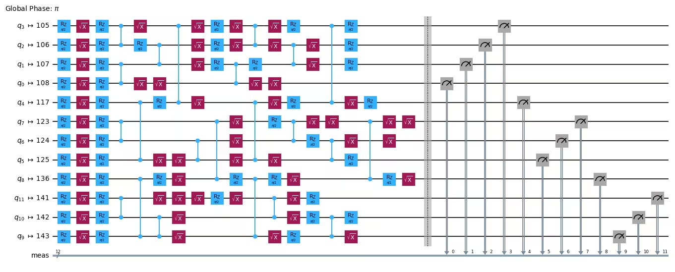
Kapag napili na ang backend at layout, i-transpile ang payload papunta sa isang instruction set architecture (ISA) circuit. Kailangan lang itakda ang layout at isalin ang mga gate patungo sa native gate set ng backend.

pm = generate_preset_pass_manager(
    optimization_level=0, backend=backend, initial_layout=layout
)
circuit_isa = pm.run(circuit)
circuit_isa.draw("mpl", fold=-1, scale=0.6)

Susunod, i-model kung paano naaapektuhan ng gate at readout noise sa backend ang execution. Tinutukoy ng noise model kung saan sa circuit ang isang check ay kumukuha ng pinakamaraming error. Ang mas tumpak na model ay nagpapabuti sa detection, ngunit kadalasan ay hindi na kailangang matutunan ito sa pamamagitan ng pag-sample sa QPU. Ang model na susunod ay nagtatantiya ng uniform depolarizing channel para sa gate at readout noise mula sa qiskit-ibm-runtime benchmark data.

noise_model = NoiseModel.from_backend(
    backend, layout, uniform_gate_noise=True
)
print(noise_model)

NoiseModel(gate_noise=0.001079865281450939, readout_noise=0.006001790364583333, idling_noise=None)

Ngayon magdagdag ng mga check sa circuit. Ang add_pauli_checks function ay kumukuha ng Clifford payload, ng listahan ng target qubits, at ng noise model. Ang ancilla_qubits argument ay nagsasabi sa function kung aling physical ancilla ang ipapares sa bawat target. Idinadagdag ang mga check ayon sa pagkakasunod-sunod ng pagpapakita ng target qubits, kaya ang final layout ng checked circuit ay layout + ancilla_qubits. Para patakbuhin ang output circuit na may mas kaunting (i) na mga check, ang final layout ay layout + ancilla_qubits[:i].

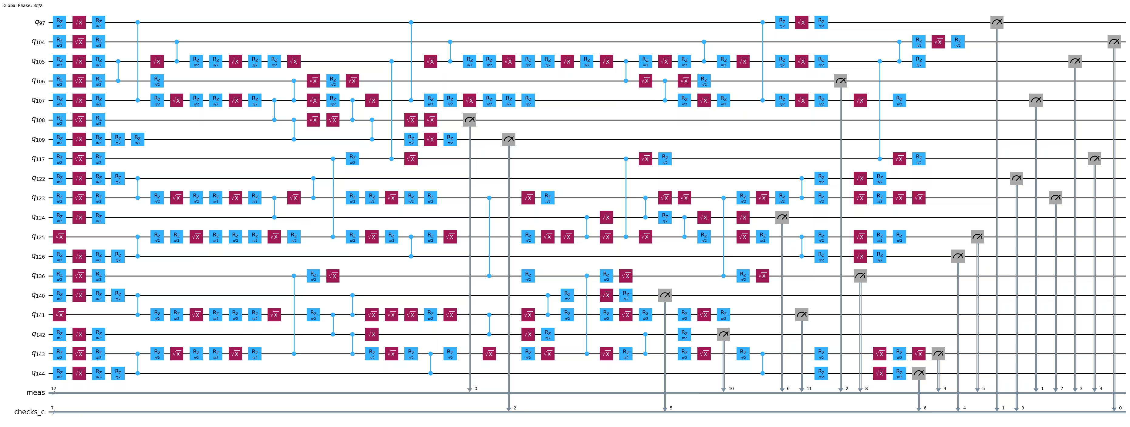
Ang output ng add_pauli_checks ay isang sequence ng mga circuit na may paparaming bilang ng mga check, mula walang check hanggang isang check sa bawat target qubit. Kinukumpirma ng visualization na ginagamit ng mga check ang tinukoy na target at ancilla pairs. Para sa mga detalye sa paghahanap ng magagandang check, tingnan ang Sections II hanggang IV ng supplementary information sa reference [1].

checked = add_pauli_checks(
    circuit_isa,
    target_qubits,
    noise_model,
    ancilla_qubits=ancilla_qubits,
    cost="gamma",
    method="windowed",
    seed=seed,
)

print(f"Physical layout of payload and ancillas: {layout + ancilla_qubits}")
print("Checked circuit:")
checked[-1].circuit.draw("mpl", fold=-1, idle_wires=False)

Physical layout of payload and ancillas: [108, 107, 106, 105, 117, 125, 124, 123, 136, 143, 142, 141, 104, 97, 109, 122, 126, 140, 144]
Checked circuit:

Step 3: Patakbuhin gamit ang Qiskit primitives

Para makita ang epekto ng gate noise, dagdagan ang lalim ng payload at mag-sample ng subset ng mga stabilizer nito. Karaniwang hindi qubit-wise commuting ang bawat stabilizer sa iba, kaya hindi valid ang iisang set ng check para sa dalawang magkaibang stabilizer. Sa halip na i-grupo ang mga stabilizer sa mga commuting set, maghanap ng magandang set ng check para sa bawat stabilizer nang hiwalay. Ang pag-sample ng mga stabilizer nang random at pantay-pantay ay nagbibigay ng unbiased fidelity estimate.

Buuin ang mas malalim na circuit at kumuha ng random na sample ng mga stabilizer nito.

depth = 24
num_stabilizers = 20
num_shots = 1_000

circuit = random_clifford_circuit(num_qubits, depth, rng)

# Build the full stabilizer group, then sample from it uniformly at random
circ_no_meas = circuit.remove_final_measurements(inplace=False)
stabilizer_group = PauliList([Pauli("I" * num_qubits)])
for generator in (
    Pauli(label) for label in Clifford(circ_no_meas).to_labels(mode="S")
):
    stabilizer_group = stabilizer_group + stabilizer_group.compose(generator)

keep = np.where(
    stabilizer_group.x.any(axis=1) | stabilizer_group.z.any(axis=1)
)[0]
chosen = np.random.default_rng(seed).choice(
    keep, size=min(num_stabilizers, len(keep)), replace=False
)
stabilizers = [stabilizer_group[int(i)] for i in chosen]

two_qubit_depth = circuit.depth(lambda x: x.operation.num_qubits == 2)
print(
    f"Sampled {len(stabilizers)} stabilizers of a {circuit.num_qubits}-qubit "
    f"circuit with two-qubit depth {two_qubit_depth}: "
    f"{{{stabilizers[0]}, {stabilizers[1]}, ...}}"
)

Sampled 20 stabilizers of a 12-qubit circuit with two-qubit depth 24: {ZXIIXZYYXIZZ, XXXYIIZYXIII, ...}

Para sa bawat sampled stabilizer, iikutin ang circuit para masukat ang stabilizer sa computational basis, i-transpile ito papunta sa backend, at maghanap ng magandang set ng check. Pinagsasama-sama at hinahalo (shuffled) ang mga target at ancilla pairs para sa bawat stabilizer para mapanatili ng bawat target ang kani-kanyang ancilla. Tandaan na naisasagawa ang mga check nang sunud-sunod ayon sa pagkakasunod-sunod ng pagbibigay ng target qubits, at hindi na binabago ang isang naisagawang check habang nagdaragdag ng mas maraming check.

noisy_circuits = []
checked_circuits = []
depths_2q = []
t0 = time.time()
for i, pauli in enumerate(tqdm(stabilizers)):
    noisy_circuits.append(pm.run(append_basis_rotation(circuit, pauli)))
    # Shuffle target and ancilla pairs together so each target keeps its ancilla
    targets, ancillas = zip(
        *random.sample(
            list(zip(target_qubits, ancilla_qubits, strict=True)),
            k=len(target_qubits),
        ),
        strict=True,
    )
    checked_circuits.append(
        add_pauli_checks(
            noisy_circuits[-1],
            list(targets),
            noise_model,
            ancilla_qubits=list(ancillas),
            cost="gamma",
            method="windowed",
            seed=seed + 1 + i,
        )
    )
    depths_2q.append(
        checked_circuits[-1][-1].circuit.depth(lambda x: len(x.qubits) == 2)
    )

print(
    f"Added {num_checks} checks to {len(stabilizers)} circuits "
    f"in {(time.time() - t0):.0f}s."
)
print(
    f"On average, two-qubit depth increased from "
    f"{circuit.depth(lambda x: len(x.qubits) == 2)} to {int(np.mean(depths_2q))} "
    f"when adding {num_checks} checks."
)

100%|██████████| 20/20 [00:15<00:00,  1.29it/s]

Added 7 checks to 20 circuits in 15s.
On average, two-qubit depth increased from 24 to 33 when adding 7 checks.

I-sample ang payload na wala pang check at ang mga checked circuit gamit ang Qiskit Aer. Ginagamit ng simulator ang parehong depolarizing model na nagrate sa mga check, kaya ang noise na tinatarget ng mga check ay ang noise na inilalapat ng simulator.

aer_nm = AerNoiseModel()
aer_nm.add_all_qubit_quantum_error(
    depolarizing_error(noise_model.gate_noise, 2), ["cz"]
)
p = noise_model.readout_noise
aer_nm.add_all_qubit_readout_error(ReadoutError([[1 - p, p], [p, 1 - p]]))
noisy_sim = AerSimulator(method="stabilizer", noise_model=aer_nm)

counts = []
for i, checked_circ_result in enumerate(tqdm(checked_circuits)):
    noisy_counts = (
        noisy_sim.run(
            noisy_circuits[i], shots=num_shots, seed_simulator=seed * i + 1
        )
        .result()
        .get_counts()
    )
    checked_counts_per_variant = []
    for k, ck in enumerate(checked_circ_result):
        variant_counts = (
            noisy_sim.run(
                ck.circuit, shots=num_shots, seed_simulator=seed * i + 2 + k
            )
            .result()
            .get_counts()
        )
        checked_counts_per_variant.append(variant_counts)
    counts.append((noisy_counts, checked_counts_per_variant))

100%|██████████| 20/20 [00:17<00:00,  1.13it/s]

Step 4: I-post-process at ibalik ang resulta sa nais na classical format

Ang bawat check ay gumagamit ng entangling gates sa pagitan ng isang ancilla at isang target. Nagsisimula ang ancilla sa $|0\rangle$, kaya sina-stabilize ng $Z_\text{anc}$ ang input nito. Ang pagpapalaganap ng $Z_\text{anc}$ pasulong sa checked circuit ay nagbubunga ng Pauli operator sa output na ang mga non-identity term ay tumutukoy sa support ng check. Pumapasa ang isang check kapag may even parity ang mga bit sa support nito. Ang isang sample ay pinananatili lamang kapag pumasa ang bawat check.

Ang get_postselection_method ng bawat CheckedCircuit ay nagbabalik ng function na nagma-map ng measured bitstring papunta sa syndrome vector. Panatilihin ang mga sample na ang syndrome ay zero para sa bawat check, at itapon ang iba. Ipinapakita ng chart na susunod na ang pagdaragdag ng mas maraming check ay nagpapababa sa postselection rate. Ang mas mababang postselection rate ay nangangailangan ng mas maraming shot para makamit ang isang target accuracy, kaya may tradeoff sa pagitan ng detection capability at sampling cost. Mukhang nagko-converge ang rate, na nagpapahiwatig na nagbibigay ng mas kaunting detection capability ang mga karagdagang check.

rate_per_variant = []
kept_per_stab = []
for i, (_, checked_counts_per_variant) in enumerate(counts):
    rates = []
    kept_at_num_checks = None
    for k, variant_counts in enumerate(checked_counts_per_variant):
        ps_fn = checked_circuits[i][k].get_postselection_method()
        kept = {
            bs: n for bs, n in variant_counts.items() if not ps_fn(bs).any()
        }
        rates.append(sum(kept.values()) / num_shots)
        if k == num_checks:
            kept_at_num_checks = kept
    rate_per_variant.append(rates)
    kept_per_stab.append(kept_at_num_checks)

max_len = max(len(s) for s in rate_per_variant)
rates_arr = np.full((len(rate_per_variant), max_len), np.nan)
for i, s in enumerate(rate_per_variant):
    rates_arr[i, : len(s)] = s
ks = np.arange(max_len)

fig, ax = plt.subplots(figsize=(8, 4))
ax.plot(ks, rates_arr.T, color="#ff8c00", alpha=0.15, linewidth=1)
ax.plot(
    ks,
    np.nanmedian(rates_arr, axis=0),
    color="black",
    linewidth=1,
    linestyle="--",
    label="median",
)
ax.set_xlabel("Checks committed")
ax.set_ylabel("Postselection rate")
ax.set_ylim((0, 1.05))
ax.set_title(
    f"Per-stabilizer postselection rate ({len(rates_arr)} stabilizers)"
)
ax.legend()
ax.grid(True, alpha=0.3)
plt.tight_layout()
plt.show()

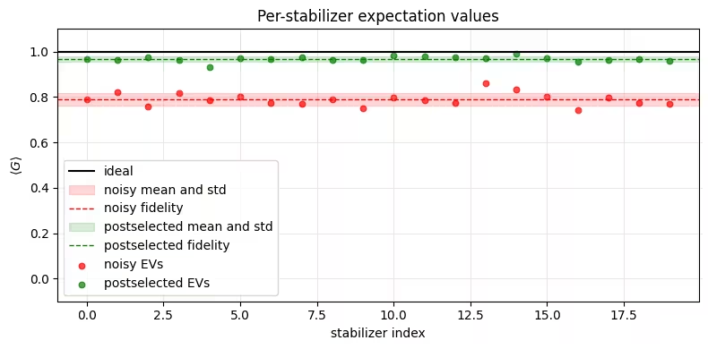
Ngayon ihambing ang fidelity ng bare noisy state kumpara sa postselected state. Ang postselecting lang ng mga sample na walang na-detect na error ay nagpapataas sa expectation value ng bawat stabilizer, at samakatuwid ay ng estimated fidelity. Ang postselected values ay gumagamit ng mas kaunting sample kaysa sa raw values, gayunpaman mas tumpak ang expectation values at mas mababa ang sampled variance. Pansinin din na ang mean postselection rate ay malapit sa noisy fidelity. Ito ang inaasahan mo kapag halos lahat ng erroneous samples ay na-detect ng mga check: ang bahagi ng mga sample na pumasa sa bawat check ay lumalapit sa bahagi ng mga sample na walang error, na siyang fidelity ng noisy state.

results = []
for i, ((noisy_counts, _), kept) in enumerate(
    zip(counts, kept_per_stab, strict=True)
):
    results.append(
        (
            expectation(noisy_counts, stabilizers[i]),
            expectation(kept, stabilizers[i]),
            sum(kept.values()) / num_shots,
        )
    )

fidelity_noisy = float(np.nanmean([r[0] for r in results]))
fidelity_postsel = float(np.nanmean([r[1] for r in results]))
psr = float(np.mean([r[2] for r in results]))
print(
    f"ideal fidelity:          1.0\n"
    f"noisy fidelity:          {fidelity_noisy:.4f}\n"
    f"postselected fidelity:   {fidelity_postsel:.4f}\n"
    f"mean postselection rate: {psr:.3f}"
)

evs_ideal = np.ones(len(results))
evs_noisy = np.array([r[0] for r in results])
evs_post = np.array([r[1] for r in results])
idx = np.arange(len(results))

def strip(ax, ys, color, label):
    m, s = np.nanmean(ys), np.nanstd(ys)
    ax.axhspan(
        m - s, m + s, color=color, alpha=0.15, label=f"{label} mean and std"
    )
    ax.axhline(
        m, color=color, linewidth=1, linestyle="--", label=f"{label} fidelity"
    )

fig, ax = plt.subplots(figsize=(8, 4))
ax.axhline(np.nanmean(evs_ideal), color="black", linewidth=1.5, label="ideal")
strip(ax, evs_noisy, "red", "noisy")
strip(ax, evs_post, "green", "postselected")
ax.scatter(idx, evs_noisy, color="red", s=22, alpha=0.7, label="noisy EVs")
ax.scatter(
    idx,
    evs_post,
    color="green",
    s=22,
    alpha=0.7,
    label="postselected EVs",
)
ax.set_xlabel("stabilizer index")
ax.set_ylabel(r"$\langle G \rangle$")
ax.set_ylim((-0.1, 1.1))
ax.set_title("Per-stabilizer expectation values")
ax.legend(loc="lower left")
ax.grid(True, alpha=0.3)
plt.tight_layout()
plt.show()

M = np.arange(1, len(results) + 1)
fig, ax = plt.subplots(figsize=(8, 4))
for ys, color, label in [
    (evs_ideal, "black", "ideal"),
    (evs_noisy, "red", "noisy"),
    (evs_post, "green", "postselected"),
]:
    cm, sem = cum_mean_sem(ys)
    ax.plot(M, cm, color=color, linewidth=1.5, label=label)
    ax.fill_between(M, cm - sem, cm + sem, color=color, alpha=0.15)
ax.set_xlabel("number of stabilizers averaged")
ax.set_ylabel("running fidelity estimate")
ax.set_title("Fidelity convergence versus number of stabilizers")
ax.legend()
ax.grid(True, alpha=0.3)
plt.tight_layout()
plt.show()

ideal fidelity:          1.0
noisy fidelity:          0.7899
postselected fidelity:   0.9679
mean postselection rate: 0.780

Ang gamma score ay nag-uulat kung gaano karami sa modeled noise channel ang nananatiling hindi na-detect ng mga check. Ang pag-plot ng gamma score laban sa bilang ng mga naisagawang check ay nagpapakita kung paano bumubuti ang detection capability habang idinaragdag ang bawat check. Ang value na 1.0 ay nangangahulugang nahuhuli ng mga check ang lahat ng modeled noise. Bumababa ang mga curve patungo sa 1.0 habang mas maraming check ang naisasagawa, na nagpapakita na ang bawat karagdagang check ay nahuhuli ang bahagi ng natitirang hindi na-detect na error.

stab_scores = [
    [variant.cost for variant in checked_circ_result]
    for checked_circ_result in checked_circuits
]
max_len = max(len(s) for s in stab_scores)
scores = np.full((len(stab_scores), max_len), np.nan)
for i, s in enumerate(stab_scores):
    scores[i, : len(s)] = s
ks = np.arange(max_len)

fig, ax = plt.subplots(figsize=(8, 4))
ax.plot(ks, scores.T, color="#4682b4", alpha=0.15, linewidth=1)
ax.plot(
    ks,
    np.nanmedian(scores, axis=0),
    color="black",
    linewidth=1,
    linestyle="--",
    label="median",
)
ax.set_xlabel("Checks committed")
ax.set_ylabel("Gamma")
ax.set_yscale("log")
ax.set_title(f"Per-stabilizer gamma curves ({len(scores)} stabilizers)")
ax.legend()
ax.grid(True, alpha=0.3, which="both")
plt.tight_layout()
plt.show()

Large-scale hardware example

Ang parehong workflow ay tumatakbo sa hardware na may mas malaki at mas malalim na payload. Muling ginagamit ng seksyong ito ang backend mula sa simulator example ngunit bumubuo ng bagong 20-qubit layout na may sariling target at ancilla pairs at pass manager, pagkatapos ay isinusumite ang mga circuit sa QPU sa iisang job. Sa laking ito, halos lahat ng shot ay nag-trigger ng kahit isang check, kaya mababa ang postselection rate, at kailangan ng bawat circuit ng malaking shot budget para sapat ang mga sample na makasurvive. Kaya naman ikinokonsentra ng halimbawang ito ang budget nito sa iilang sampled stabilizer; ito ay unbiased fidelity estimate pa rin, ngunit mas magaspang (coarser) kaysa sa average ng simulator example sa maraming stabilizer.

May isang bagay na nagbabago kumpara sa simulator example: sa halip na magtantiya ng uniform depolarizing channel mula sa calibration data, ang seksyong ito ay natututo ng noise model gamit ang NoiseLearner at bumubuo ng qiskit-paulice model mula sa resulta gamit ang NoiseModel.from_pauli_lindblad_maps. Isang natutunang Pauli-Lindblad model ang kumukuha sa spatial structure ng noise sa partikular na layout na ito, sa halip na ipagpalagay na pantay-pantay ang noise sa bawat edge, kaya na-rate ang placement ng check laban sa noise na mas kapareho ng nakakaapekto sa QPU. Ang pagkatuto ng noise ay nangangailangan ng pag-sample sa QPU at dapat isaalang-alang sa kabuuang QPU sampling budget.

Itinatakda ng mga parameter na susunod ang bilang ng qubit, ang lalim, ang bilang ng stabilizer, at ang bilang ng shot. I-scale ang hw_num_shots gamit ang inverse ng postselection rate: sa 3% na rate, ang 40,000 shots ay nag-iiwan ng humigit-kumulang 1,200 postselected samples kada circuit. Dagdagan ang hw_num_stabilizers para sa mas tumpak na fidelity estimate sa halagang mas maraming circuit kada job, na bawat isa ay nangangailangan ng parehong shot budget.

Steps 1-4 (naka-compress sa isang code block)

Ang sumusunod na cell ay pinapatakbo ang parehong apat na hakbang gaya ng simulator example. Binubuo nito ang mas malaking payload at kumukuha ng sample ng iilang stabilizer (step 1); pumipili ng layout, natututo ng noise model dito, at hinahanap ang fully checked circuit para sa bawat stabilizer (step 2); nagsusumite ng isang Sampler job na naglalaman ng parehong bare at checked circuits (step 3); at nagpo-postselect sa checked counts para ihambing ang noisy at postselected fidelity estimates, kada stabilizer at sa average (step 4). Sa laking ito, imposible nang i-enumerate ang buong stabilizer group tulad ng simulator example, kaya ang cell ay kumukuha ng random na subsample ng mga stabilizer para kalkulahin ang tantiya ng fidelity.

Pansinin na gumagawa ng mas marami ang step 2 dito kaysa sa simulator example: ang pagkatuto ng noise model ay nagsusumite ng sarili nitong NoiseLearner job bago ang Sampler job, kaya ang cell ay nagpapatakbo ng dalawang job sa kabuuan. May mga tag itong TUT_ASPC_LEARN at TUT_ASPC para mahanap mo sila sa ibang pagkakataon. Tingnan ang Organize and search by job tags para sa karagdagang impormasyon tungkol sa pag-tag ng mga job.

# -------------------------Step 1: build a larger payload and sample stabilizers-------------------------
hw_num_qubits = 20
hw_depth = 36
hw_num_stabilizers = 10
hw_num_shots = 40_000

hw_circuit = random_clifford_circuit(hw_num_qubits, hw_depth, rng)
hw_no_meas = hw_circuit.remove_final_measurements(inplace=False)

# Enumerating all 2^n stabilizers is infeasible at this size, so draw each
# stabilizer by composing a random subset of the group generators
hw_generators = [
    Pauli(label) for label in Clifford(hw_no_meas).to_labels(mode="S")
]
sample_rng = np.random.default_rng(seed)
hw_stabilizers = []
while len(hw_stabilizers) < hw_num_stabilizers:
    mask = sample_rng.integers(0, 2, hw_num_qubits).astype(bool)
    if not mask.any():
        continue  # skip the identity
    stabilizer = Pauli("I" * hw_num_qubits)
    for generator, chosen in zip(hw_generators, mask, strict=True):
        if chosen:
            stabilizer = stabilizer.compose(generator)
    hw_stabilizers.append(stabilizer)

# -------------------------Step 2: find a 20-qubit layout, learn its noise, and add checks-------------------------
# A single bad coupler or bad-readout qubit on the path drags every
# stabilizer down, so search harder and with tighter error thresholds
hw_layout = find_check_layout(
    backend,
    hw_num_qubits,
    rng,
    num_trials=500,
    max_gate_error=0.015,
    max_readout_error=0.05,
)
hw_target_qubits, hw_ancilla_qubits = get_check_qubits(backend, hw_layout)
hw_pm = generate_preset_pass_manager(
    optimization_level=0, backend=backend, initial_layout=hw_layout
)
print(f"Layout with {len(hw_target_qubits)} check pairs: {hw_layout}")

# ----- learn a Pauli-Lindblad noise model on this layout -----
# The simulator example scored checks against a uniform depolarizing channel
# inferred from calibration data. Here, learn the noise instead: NoiseLearner
# runs its own job on the QPU and returns a Pauli-Lindblad channel per unique
# entangling layer, so the checks are placed against the noise this layout
# actually has, including its spatial structure. All the sampled stabilizers
# share the same entangling layers and differ only in their final basis
# rotation, so learning on the bare payload covers all of them.
learner = NoiseLearner(
    mode=backend,
    options={
        "max_layers_to_learn": 4,
        "num_randomizations": 32,
        "shots_per_randomization": 128,
        "environment": {"job_tags": ["TUT_ASPC_LEARN"]},
    },
)
learner_job = learner.run([hw_pm.run(hw_circuit)])
print(f"Submitted noise-learner job {learner_job.job_id()}")
hw_layer_errors = learner_job.result().data

# To see how much the learned model helps, swap the next line for the
# simulator example's uniform model - a one-line change:
# hw_noise_model = NoiseModel.from_backend(backend, hw_layout, uniform_gate_noise=True)
hw_noise_model = learned_noise_model(hw_layer_errors, hw_layout)
# NoiseLearner characterizes gate noise only, so keep the readout estimate
# from calibration data rather than leaving it unset
hw_noise_model.readout_noise = NoiseModel.from_backend(
    backend, hw_layout, uniform_gate_noise=True
).readout_noise
print(
    f"Learned {len(hw_layer_errors)} layers; "
    f"readout noise {hw_noise_model.readout_noise:.5f}"
)

# ----- add the fully checked circuit per stabilizer -----
hw_noisy_circuits = []
hw_checked_circuits = []
for i, pauli in enumerate(tqdm(hw_stabilizers)):
    bare = hw_pm.run(append_basis_rotation(hw_circuit, pauli))
    hw_noisy_circuits.append(bare)
    variants = add_pauli_checks(
        bare,
        hw_target_qubits,
        hw_noise_model,
        ancilla_qubits=hw_ancilla_qubits,
        cost="gamma",
        method="windowed",
        seed=seed + 1 + i,
    )
    hw_checked_circuits.append(variants[-1])  # keep the fully checked circuit

# -------------------------Step 3: submit one Sampler job with the bare and checked circuits-------------------------
sampler = Sampler(mode=backend)
sampler.options.default_shots = hw_num_shots
sampler.options.environment.job_tags = ["TUT_ASPC"]

pubs = hw_noisy_circuits + [cc.circuit for cc in hw_checked_circuits]
job = sampler.run(pubs)
print(f"Submitted job {job.job_id()} with {len(pubs)} circuits")

# -------------------------Step 4: postselect and compare fidelity-------------------------
result = job.result()
n_stab = len(hw_stabilizers)

hw_results = []
for i in range(n_stab):
    noisy_counts = result[i].join_data().get_counts()
    checked_counts = result[n_stab + i].join_data().get_counts()
    ps_fn = hw_checked_circuits[i].get_postselection_method()
    kept = {bs: c for bs, c in checked_counts.items() if not ps_fn(bs).any()}
    hw_results.append(
        (
            expectation(noisy_counts, hw_stabilizers[i]),
            expectation(kept, hw_stabilizers[i]),
            sum(kept.values()) / sum(checked_counts.values()),
        )
    )

hw_fidelity_noisy = float(np.nanmean([r[0] for r in hw_results]))
hw_fidelity_postsel = float(np.nanmean([r[1] for r in hw_results]))
hw_psr = float(np.mean([r[2] for r in hw_results]))
print(
    f"noisy fidelity estimate:        {hw_fidelity_noisy:.4f}\n"
    f"postselected fidelity estimate: {hw_fidelity_postsel:.4f}\n"
    f"mean postselection rate:        {hw_psr:.4f} "
    f"(~{int(round(hw_psr * hw_num_shots))} kept shots per circuit)"
)

# Per-stabilizer breakdown. The postselection rate varies from stabilizer to
# stabilizer, so a stabilizer whose postselected value barely moves is usually
# one whose checks rejected little; the kept-shot count says how much of the
# gap is statistics rather than signal.
print("\nper-stabilizer results:")
print(
    f"{'idx':>3}  {'noisy':>8}  {'postsel':>8}  {'psr':>7}  {'kept shots':>10}"
)
for i, (noisy, post, psr_i) in enumerate(hw_results):
    print(
        f"{i:>3}  {noisy:>8.4f}  {post:>8.4f}  {psr_i:>7.4f}  "
        f"{int(round(psr_i * hw_num_shots)):>10}"
    )

hw_noisy = np.array([r[0] for r in hw_results])
hw_post = np.array([r[1] for r in hw_results])
idx = np.arange(n_stab)

fig, ax = plt.subplots(figsize=(9, 4))
ax.axhline(1.0, color="black", linewidth=1.5, label="ideal")
strip(ax, hw_noisy, "red", "noisy")
strip(ax, hw_post, "green", "postselected")
ax.scatter(idx, hw_noisy, color="red", s=22, alpha=0.7, label="noisy EVs")
ax.scatter(
    idx,
    hw_post,
    color="green",
    s=22,
    alpha=0.7,
    label="postselected EVs",
)
ax.set_xlabel("stabilizer index")
ax.set_ylabel(r"$\langle G \rangle$")
ax.set_ylim((-0.1, 1.1))
ax.set_xticks(idx)
ax.set_title("Per-stabilizer expectation values on hardware")
# Outside the axes so it cannot hide a data point
ax.legend(loc="center left", bbox_to_anchor=(1.02, 0.5), frameon=False)
ax.grid(True, alpha=0.3)
plt.tight_layout()
plt.show()

Layout with 11 check pairs: [153, 152, 151, 138, 131, 130, 129, 118, 109, 110, 111, 98, 91, 90, 89, 78, 69, 70, 71, 58]
Submitted noise-learner job d9f4mncjeosc73fjfmkg

Learned 4 layers; readout noise 0.00470

100%|██████████| 10/10 [01:01<00:00,  6.18s/it]

Submitted job d9f4s04jeosc73fjftkg with 20 circuits
noisy fidelity estimate:        0.3685
postselected fidelity estimate: 0.6869
mean postselection rate:        0.2851 (~11404 kept shots per circuit)

per-stabilizer results:
idx     noisy   postsel      psr  kept shots
  0    0.3769    0.6918   0.3247       12987
  1    0.3745    0.6760   0.2999       11995
  2    0.3659    0.6389   0.3549       14196
  3    0.3821    0.7060   0.2660       10641
  4    0.3653    0.7475   0.2531       10124
  5    0.3752    0.7022   0.2698       10791
  6    0.3508    0.7144   0.2711       10842
  7    0.3485    0.7087   0.2381        9523
  8    0.3825    0.6289   0.2928       11711
  9    0.3630    0.6549   0.2808       11232

Para sa mga circuit ng laking ito, karamihan sa mga sample ay may kahit isang na-detect na error, kaya maliit ang postselection rate at itinatapon ng postselection ang karamihan ng mga shot. Ang mga sample na pumasa sa bawat check ay nagbibigay ng mas mahusay na expectation value kaysa sa bare circuit, at ang per-stabilizer values ay malinaw na naiiba mula sa noisy baseline. Para paigtingin ang fidelity estimate, mag-sample ng mas maraming stabilizer gamit ang parehong per-circuit shot budget. Para itaas ang postselection rate, bawasan ang circuit depth o magsagawa ng mas kaunting check; para umangat sa mas malalaking payload, i-scale ang shot budget gamit ang inverse ng postselection rate.

Mga susunod na hakbang

Recommendations

Kung interesado ka sa gawaing ito, maaaring interesado ka rin sa mga sumusunod na materyal:

• Ang tutorial sa repetition codes para sa panimula sa quantum error correction.

• Ang qiskit-paulice documentation para sa buong check-finding API, at ang GitHub repository ng package para sa source code.

• Ang papel Low-overhead error detection with spacetime codes para sa teorya sa likod ng mga check.

References

• [1] Martiel, S., & Javadi-Abhari, A. (2025). Low-overhead error detection with spacetime codes. arXiv preprint arXiv:2504.15725.

• [2] van den Berg, E., Bravyi, S., Gambetta, J. M., Jurcevic, P., Maslov, D., & Temme, K. (2023). Single-shot error mitigation by coherent Pauli checks. Physical Review Research, 5(3), 033193.