Quantum algorithms: Pagtatantya ng phase

tala

Kento Ueda (15 Mayo 2024)

Ang notebook na ito ay nagbibigay ng mga pangunahing konsepto at implementasyon ng Quantum Fourier Transformation (QFT) at Quantum Phase Estimation (QPE).

I-download ang pdf ng orihinal na lektura. Tandaan na ang ilang code snippet ay maaaring maging deprecated dahil ito ay mga static na larawan.

Ang tinatayang QPU time para patakbuhin ang eksperimentong ito ay 7 segundo.

1. Panimula

Quantum Fourier Transformation (QFT)

Ang Quantum Fourier Transformation ay ang quantum na katumbas ng klasikal na discrete Fourier transform. Ito ay isang linear na transformasyon na inilalapat sa mga quantum state, na nag-map ng mga computational basis patungo sa kanilang mga representasyon sa Fourier basis. Mahalaga ang QFT sa maraming quantum algorithm, dahil nagbibigay ito ng mahusay na paraan upang makuha ang impormasyon ng periodicity mula sa mga quantum state. Maaaring ipatupad ang QFT gamit ang $O(N^2)$ na operasyon sa pamamagitan ng mga quantum gate tulad ng Hadamard gate at Control-Phase gate para sa $N$ qubit, na nagbibigay ng exponential na pagbilis kumpara sa klasikal na Fourier transformation.

• Mga Aplikasyon: Ito ay isang pundasyon ng mga quantum algorithm tulad ng Shor's algorithm para sa pag-factor ng malalaking integer at discrete logarithm.

Quantum Phase Estimation (QPE)

Ang Quantum Phase Estimation ay isang quantum algorithm na ginagamit upang matantya ang phase na nauugnay sa eigenvector ng isang unitary operator. Ang algorithm na ito ay nagsisilbing tulay sa pagitan ng mga abstract na mathematical na katangian ng mga quantum state at ng kanilang mga computational na aplikasyon.

• Mga Aplikasyon: Kaya nitong lutasin ang mga problema tulad ng paghanap ng mga eigenvalue ng unitary matrix at pag-simulate ng mga quantum system.

Sama-sama, ang QFT at QPE ang bumubuo ng mahahalagang pundasyon ng maraming quantum algorithm na nalulutas ng mga problemang hindi magagawa ng mga klasikal na computer. Sa pagtatapos ng notebook na ito, magkakaroon ka ng pag-unawa kung paano ipinapatupad ang mga pamamaraang ito.

2. Mga Pangunahing Kaalaman sa Quantum Fourier Transformation (QFT)

# Added by doQumentation — required packages for this notebook
!pip install -q numpy qiskit qiskit-aer qiskit-ibm-runtime

from qiskit import QuantumCircuit, QuantumRegister, ClassicalRegister
from qiskit_aer import AerSimulator
from qiskit.visualization import plot_histogram, plot_bloch_multivector
from qiskit.quantum_info import Statevector
from qiskit.transpiler.preset_passmanagers import generate_preset_pass_manager
from qiskit_ibm_runtime import Sampler

from numpy import pi

Mula sa pagkakatulad sa discrete Fourier transform, ang QFT ay kumikilos sa isang quantum state na $\vert X\rangle = \sum_{j=0}^{N-1} x_j \vert j \rangle$ para sa $N$ qubit at nima-map ito sa quantum state na $\vert Y\rangle = \sum_{k=0}^{N-1} y_k \vert k \rangle$.

$$QFT_{N}: \vert j \rangle \mapsto \frac{1}{\sqrt{N}}\sum_{k=0}^{N-1}\omega_N^{jk} \vert k \rangle$$

kung saan ang $\omega_N^{jk} = e^{2\pi i \frac{jk}{N}}$.

O ang representasyon sa unitary matrix:

$$U_{QFT} = \frac{1}{\sqrt{N}} \sum_{j=0}^{N-1} \sum_{k=0}^{N-1} \omega_N^{jk} \vert k \rangle \langle j \vert$$

2.1. Intuisyon

Ang quantum Fourier transform (QFT) ay nagtatransforma sa pagitan ng dalawang basis: ang computational (Z) basis, at ang Fourier basis. Pero ano ang ibig sabihin ng Fourier basis sa kontekstong ito? Malamang na naalala mo na ang Fourier transform na $F(\omega)$ ng isang function na $f(x)$ ay naglalarawan ng convolution ng $f(x)$ sa isang sinusoidal function na may frequency na $\omega$. Sa simpleng salita: ang Fourier transform ay isang function na naglalarawan kung gaano karaming bawat frequency $\omega$ ang kailangan natin upang bumuo ng isang function na $f(x)$ mula sa mga sine function (o cosine function). Upang mas maunawaan ang ibig sabihin ng QFT sa kontekstong ito, tingnan ang mga step na larawan sa ibaba na nagpapakita ng isang numerong naka-encode sa binary gamit ang apat na qubit:

Sa computational basis, iniimbak natin ang mga numero sa binary gamit ang mga state na $|0\rangle$ at $|1\rangle$.

Pansinin ang frequency kung saan nagbabago ang iba't ibang qubit; ang pinakakaliwa na qubit ay nag-i-flip sa bawat dagdag ng numero, ang susunod ay bawat 2 na dagdag, ang ikatlo ay bawat 4 na dagdag, at iba pa.

Kung mag-apply tayo ng quantum Fourier transform sa mga state na ito, magma-map tayo:

$$|\text{State in Computational Basis}\rangle \quad \xrightarrow[]{\text{QFT}} \quad |\text{State in Fourier Basis}\rangle$$ $$\text{QFT}|x\rangle = |\widetilde{x}\rangle$$

(Kadalasang tinutukoy natin ang mga state sa Fourier basis gamit ang tilde (~)).

Sa Fourier basis, iniimbak natin ang mga numero gamit ang iba't ibang rotasyon sa paligid ng Z-axis:

IFRAME

Ang numerong gusto nating itago ang nagdidikta ng anggulo kung saan inii-rotate ang bawat qubit sa paligid ng Z-axis. Sa state na $|\widetilde{0}\rangle$, lahat ng qubit ay nasa state na $|{+}\rangle$. Gaya ng nakikita sa halimbawa sa itaas, upang i-encode ang state na $|\widetilde{5}\rangle$ sa 4 na qubit, ini-rotate natin ang pinakakaliwang qubit ng $\tfrac{5}{2^n} = \tfrac{5}{16}$ na buong ikot ($\tfrac{5}{16}\times 2\pi$ radian). Ang susunod na qubit ay double nito ($\tfrac{10}{16}\times 2\pi$ radian, o $10/16$ na buong ikot), at doble rin ang anggulo para sa qubit pagkatapos, at iba pa.

Muli, pansinin ang frequency kung saan nagbabago ang bawat qubit. Ang pinakakaliwang qubit (qubit 0) sa kasong ito ay may pinakamababang frequency, at ang pinakakanan ang may pinakamataas.

2.2 Halimbawa: 1-qubit QFT

Isaalang-alang natin ang kaso ng $N = 2^1 = 2$.

Ang unitary matrix ay maaaring isulat:

$$\begin{aligned} U_{QFT} & = \frac{1}{\sqrt{2}} \sum_{j=0}^{1} \sum_{k=0}^{1} \omega_2^{jk} \vert k \rangle \langle j \vert \\ & = \frac{1}{\sqrt{2}} (\omega_2^{0} \vert 0 \rangle \langle 0 \vert + \omega_2^{0} \vert 0 \rangle \langle 1 \vert + \omega_2^{0} \vert 1 \rangle \langle 0 \vert + \omega_2^{1} \vert 1 \rangle \langle 1 \vert) \\ & = \frac{1}{\sqrt{2}} (\vert 0 \rangle \langle 0 \vert + \vert 0 \rangle \langle 1 \vert + \vert 1 \rangle \langle 0 \vert - \vert 1 \rangle \langle 1 \vert) \\ & = H \end{aligned}$$

Ang operasyong ito ay resulta ng pag-apply ng Hadamard gate ($H$).

2.3 Representasyon ng produkto ng QFT

I-generalize natin ang isang transformasyon para sa $N = 2^n$, ang $QFT_{N}$ na kumikilos sa state na $\vert x \rangle = \vert x_1\ldots x_n \rangle$.

$$\begin{aligned} QFT_N\vert x \rangle & = \frac{1}{\sqrt{N}} \sum_{y=0}^{N-1}\omega_N^{xy} \vert y \rangle \\ & = \frac{1}{\sqrt{N}} \sum_{y=0}^{N-1} e^{2 \pi i xy / 2^n} \vert y \rangle ~\text{since}\: \omega_N^{xy} = e^{2\pi i \frac{xy}{N}} \:\text{and}\: N = 2^n \\ & = \frac{1}{\sqrt{N}} \sum_{y=0}^{N-1} e^{2 \pi i \left(\sum_{k=1}^n y_k/2^k\right) x} \vert y_1 \ldots y_n \rangle \:\text{rewriting in fractional binary notation}\: y = y_1\ldots y_n, y/2^n = \sum_{k=1}^n y_k/2^k \\ & = \frac{1}{\sqrt{N}} \sum_{y=0}^{N-1} \prod_{k=1}^n e^{2 \pi i x y_k/2^k } \vert y_1 \ldots y_n \rangle \:\text{after expanding the exponential of a sum to a product of exponentials,} \\ & = \frac{1}{\sqrt{N}} \bigotimes_{k=1}^n \left(\vert0\rangle + e^{2 \pi i x /2^k } \vert1\rangle \right) \:\text{after rearranging the sum and products, and expanding} \sum_{y=0}^{N-1} = \sum_{y_1=0}^{1}\sum_{y_2=0}^{1}\ldots\sum_{y_n=0}^{1} \\ & = \frac{1}{\sqrt{N}} \left(\vert0\rangle + e^{\frac{2\pi i}{2}x} \vert1\rangle\right) \otimes \left(\vert0\rangle + e^{\frac{2\pi i}{2^2}x} \vert1\rangle\right) \otimes \ldots \otimes \left(\vert0\rangle + e^{\frac{2\pi i}{2^{n-1}}x} \vert1\rangle\right) \otimes \left(\vert0\rangle + e^{\frac{2\pi i}{2^n}x} \vert1\rangle\right) \end{aligned}$$

2.4 Halimbawa: Pagbuo ng Circuit ng 3-qubit QFT

Mula sa paglalarawan sa itaas, maaaring hindi malinaw kung paano bumuo ng QFT circuit. Sa ngayon, tandaan lamang na inaasahan nating ang tatlong qubit ay may mga phase na nag-e-evolve sa iba't ibang "bilis". Ang pag-unawa kung paano ito isasalin sa isang circuit ay iniiwan bilang ehersisyo para sa mambabasa. Mayroon maraming diagram at halimbawa sa lecture pdf. Ang karagdagang mapagkukunan ay kinabibilangan ng araling ito mula sa kursong Fundamentals of quantum algorithms.

Ipapakita natin ang QFT gamit lamang ang mga simulator, at samakatuwid hindi natin gagamitin ang Qiskit patterns framework hanggang sa lumipat tayo sa quantum phase estimation.

# Prepare for 3 qubits circuit
qr = QuantumRegister(3)
cr = ClassicalRegister(3)
qc = QuantumCircuit(qr, cr)

qc.h(2)
qc.cp(pi / 2, 1, 2)  # Controlled-phase gate from qubit 1 to qubit 2
qc.cp(pi / 4, 0, 2)  # Controlled-phase gate from qubit 0 to qubit 2
qc.draw(output="mpl")

qc.h(1)
qc.cp(pi / 2, 0, 1)  # Controlled-phase gate from qubit 0 to qubit 1

qc.draw(output="mpl")

qc.h(0)

qc.draw(output="mpl")

qc.swap(0, 2)

qc.draw(output="mpl")

Susubukan nating i-apply ang QFT sa $|5\rangle$ bilang halimbawa.

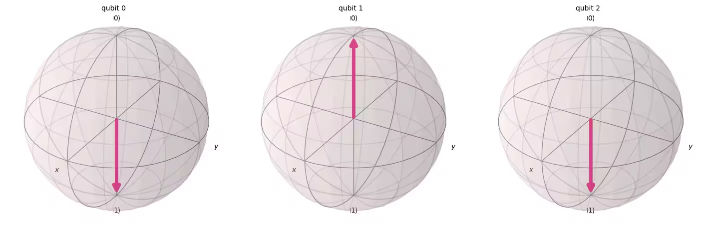
Una, kinukumpirma natin ang binary notation ng integer 5 at ginagawa ang circuit na nag-e-encode ng state 5:

bin(5)

'0b101'

qc = QuantumCircuit(3)

qc.x(0)
qc.x(2)
qc.draw(output="mpl")

Sinusuri natin ang mga quantum state gamit ang Aer simulator:

statevector = Statevector(qc)
plot_bloch_multivector(statevector)

Sa wakas, idinaragdag natin ang QFT at tinitingnan ang panghuling state ng ating mga qubit:

qc.h(2)
qc.cp(pi / 2, 1, 2)
qc.cp(pi / 4, 0, 2)

qc.h(1)
qc.cp(pi / 2, 0, 1)

qc.h(0)

qc.swap(0, 2)

qc.draw(output="mpl")

statevector = Statevector(qc)
plot_bloch_multivector(statevector)

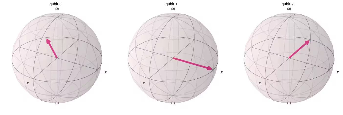
Makikita natin na gumana nang tama ang ating QFT function. Nai-rotate ang Qubit 0 ng $\tfrac{5}{8}$ ng isang buong ikot, ang qubit 1 ng $\tfrac{10}{8}$ na buong ikot (katumbas ng $\tfrac{1}{4}$ ng isang buong ikot), at ang qubit 2 ng $\tfrac{20}{8}$ na buong ikot (katumbas ng $\tfrac{1}{2}$ ng isang buong ikot).

2.5 Ehersisyo: QFT

(1) Ipatupad ang QFT ng 4 na qubit.

##your code goes here##

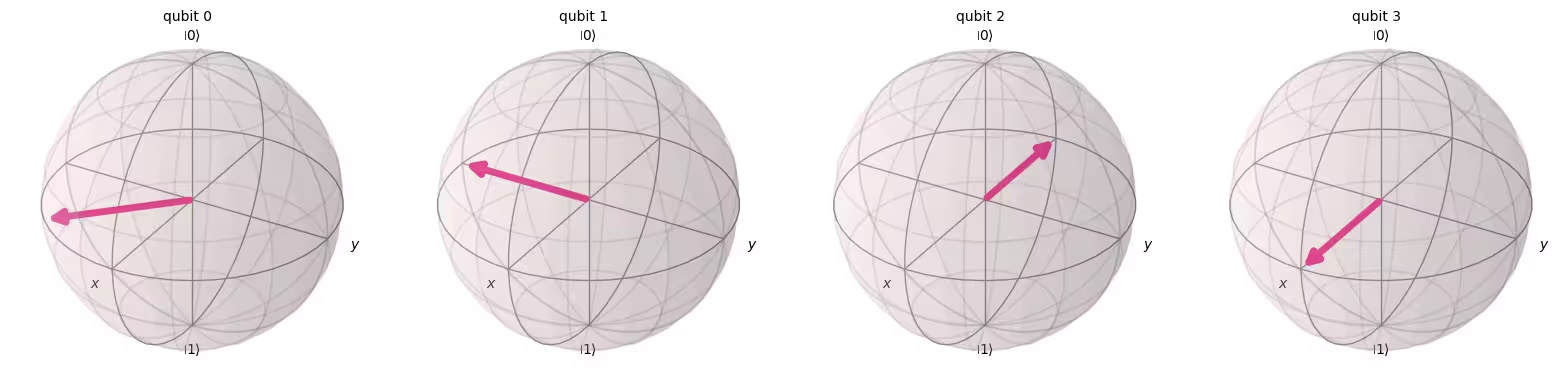
(2) I-apply ang QFT sa $|14\rangle$, i-simulate at i-plot ang statevector gamit ang Bloch sphere.

##your code goes here##

Solusyon ng ehersisyo: QFT

(1)

qr = QuantumRegister(4)
cr = ClassicalRegister(4)
qc = QuantumCircuit(qr, cr)

qc.h(3)
qc.cp(pi / 2, 2, 3)
qc.cp(pi / 4, 1, 3)
qc.cp(pi / 8, 0, 3)

qc.h(2)
qc.cp(pi / 2, 1, 2)
qc.cp(pi / 4, 0, 2)

qc.h(1)
qc.cp(pi / 2, 0, 1)

qc.h(0)

qc.swap(0, 3)
qc.swap(1, 2)

qc.draw(output="mpl")

(2)

bin(14)

'0b1110'

qc = QuantumCircuit(4)

qc.x(1)
qc.x(2)
qc.x(3)
qc.draw("mpl")

qc.h(3)
qc.cp(pi / 2, 2, 3)
qc.cp(pi / 4, 1, 3)
qc.cp(pi / 8, 0, 3)

qc.h(2)
qc.cp(pi / 2, 1, 2)
qc.cp(pi / 4, 0, 2)

qc.h(1)
qc.cp(pi / 2, 0, 1)
qc.h(0)

qc.swap(0, 3)
qc.swap(1, 2)

qc.draw(output="mpl")

statevector = Statevector(qc)
plot_bloch_multivector(statevector)

3. Mga Pangunahing Kaalaman sa Quantum Phase Estimation (QPE)

Dahil sa isang unitary na operasyon na $U$, tinatantya ng QPE ang $\theta$ sa $U\vert\psi \rangle =e^{\boldsymbol{2\pi i} \theta }|\psi \rangle$ dahil ang $U$ ay unitary, lahat ng eigenvalue nito ay may norm na 1.

3.1 Pamamaraan

1. Setup

Ang $\vert\psi\rangle$ ay nasa isang hanay ng mga qubit register. Ang karagdagang hanay ng $n$ qubit ay bumubuo ng counting register kung saan itatago natin ang value na $2^n\theta$:

$$|\psi_0\rangle = \lvert 0 \rangle^{\otimes n} \lvert \psi \rangle$$

2. Superposition

Mag-apply ng $n$-bit na Hadamard gate na operasyon na $H^{\otimes n}$ sa counting register:

$$|\psi_1\rangle = {\frac {1}{2^{\frac {n}{2}}}}\left(|0\rangle +|1\rangle \right)^{\otimes n} \lvert \psi \rangle$$

3. Mga Controlled Unitary na Operasyon

Kailangan nating ipakilala ang controlled unitary na $CU$ na nag-a-apply ng unitary operator na $U$ sa target register kung ang kaukulang control bit nito ay $|1\rangle$ lamang. Dahil ang $U$ ay isang unitary operator na may eigenvector na $|\psi\rangle$ kung saan $U|\psi \rangle =e^{\boldsymbol{2\pi i} \theta }|\psi \rangle$, ibig sabihin nito:

$$U^{2^{j}}|\psi \rangle =U^{2^{j}-1}U|\psi \rangle =U^{2^{j}-1}e^{2\pi i\theta }|\psi \rangle =\cdots =e^{2\pi i2^{j}\theta }|\psi \rangle$$

3.2 Halimbawa: T-gate QPE

Gamitin natin ang $T$ gate bilang halimbawa ng QPE at tantiyahin ang phase nito na $\theta$.

$$T|1\rangle = \begin{pmatrix} 1 & 0\\ 0 & e^\frac{i\pi}{4}\\ \end{pmatrix} \begin{pmatrix} 0\\ 1\\ \end{pmatrix} = e^\frac{i\pi}{4}|1\rangle$$

Inaasahan nating mahanap:

$$\theta = \frac{1}{8}$$

kung saan

$$T|1\rangle = e^{2i\pi\theta}|1\rangle$$

Ini-initialize natin ang $\vert\psi\rangle = \vert1\rangle$ ng eigenvector ng $T$ gate sa pamamagitan ng pag-apply ng $X$ gate:

qpe = QuantumCircuit(4, 3)
qpe.x(3)
qpe.draw(output="mpl")

Susunod, nag-a-apply tayo ng mga Hadamard gate sa mga counting qubit:

for qubit in range(3):
    qpe.h(qubit)
qpe.draw(output="mpl")

Ginagawa natin ang mga controlled unitary na operasyon:

repetitions = 1
for counting_qubit in range(3):
    for i in range(repetitions):
        qpe.cp(pi / 4, counting_qubit, 3)  # This is C-U
    repetitions *= 2
qpe.draw(output="mpl")

Ina-apply natin ang inverse quantum Fourier transformation upang i-convert ang state ng counting register, pagkatapos ay sinusukat ang counting register:

from qiskit.circuit.library import QFT

# Apply inverse QFT
qpe.append(QFT(3, inverse=True), [0, 1, 2])
qpe.draw(output="mpl")

for n in range(3):
    qpe.measure(n, n)
qpe.draw(output="mpl")

Maaari tayong mag-simulate gamit ang Aer simulator:

aer_sim = AerSimulator()
shots = 2048

pm = generate_preset_pass_manager(backend=aer_sim, optimization_level=1)
t_qpe = pm.run(qpe)

sampler = Sampler(mode=aer_sim)
job = sampler.run([t_qpe], shots=shots)
result = job.result()
answer = result[0].data.c.get_counts()

plot_histogram(answer)

Makikita natin na nakakuha tayo ng isang resulta (001) nang may katiyakan, na nagsasalin sa decimal: 1. Kailangan na nating hatiin ang ating resulta (1) sa $2^n$ upang makuha ang $\theta$:

$$\theta = \frac{1}{2^3} = \frac{1}{8}$$

Ang Shor's algorithm ay nagbibigay-daan sa atin na mag-factorize ng isang numero sa pamamagitan ng pagbuo ng circuit na may hindi kilalang $\theta$ at pagkuha ng $\theta$.

3.3 Ehersisyo

Tantiyahin ang $\theta = 1/3$ gamit ang 3 qubit para sa pagbibilang at isang qubit para sa isang eigenvector.

$P|1\rangle = e^{i\lambda}|1\rangle$. Dahil gusto nating ipatupad ang $U|1\rangle = e^{2\pi i \tfrac{1}{3}}|1\rangle$, kailangan nating itakda ang $\lambda = \tfrac{2 \pi}{3}$.

##your code goes here##

Solusyon ng ehersisyo: $\theta = 1/3$

# Create and set up circuit
qpe = QuantumCircuit(4, 3)

# Apply H-Gates to counting qubits:
for qubit in range(3):
    qpe.h(qubit)

# Prepare our eigenstate |psi>:
qpe.x(3)

# Do the controlled-U operations:
angle = 2 * pi / 3
repetitions = 1
for counting_qubit in range(3):
    for i in range(repetitions):
        qpe.cp(angle, counting_qubit, 3)
    repetitions *= 2

# Do the inverse QFT:
qpe.append(QFT(3, inverse=True), [0, 1, 2])

for n in range(3):
    qpe.measure(n, n)

qpe.draw(output="mpl")

aer_sim = AerSimulator()
shots = 4096

pm = generate_preset_pass_manager(backend=aer_sim, optimization_level=1)
t_qpe = pm.run(qpe)

sampler = Sampler(mode=aer_sim)
job = sampler.run([t_qpe], shots=shots)
result = job.result()
answer = result[0].data.c.get_counts()

plot_histogram(answer)

4. Pagpapatakbo gamit ang Qiskit Runtime Sampler Primitive

Gagawa tayo ng QPE gamit ang tunay na quantum device at susundin ang 4 na hakbang ng Qiskit patterns.

1. I-map ang problema sa quantum-native na format
2. I-optimize ang mga circuit
3. Patakbuhin ang target circuit
4. I-post-process ang mga resulta

from qiskit_ibm_runtime import QiskitRuntimeService
from qiskit_ibm_runtime import Sampler

# Loading your IBM Quantum® account(s)

service = QiskitRuntimeService()

4.1 Hakbang 1: I-map ang problema sa mga quantum circuit at operator

qpe = QuantumCircuit(4, 3)
qpe.x(3)
for qubit in range(3):
    qpe.h(qubit)
repetitions = 1
for counting_qubit in range(3):
    for i in range(repetitions):
        qpe.cp(pi / 4, counting_qubit, 3)  # This is C-U
    repetitions *= 2
qpe.append(QFT(3, inverse=True), [0, 1, 2])
for n in range(3):
    qpe.measure(n, n)
qpe.draw(output="mpl")

backend = service.least_busy(simulator=False, operational=True, min_num_qubits=4)

print(backend)

<IBMBackend('ibm_strasbourg')>

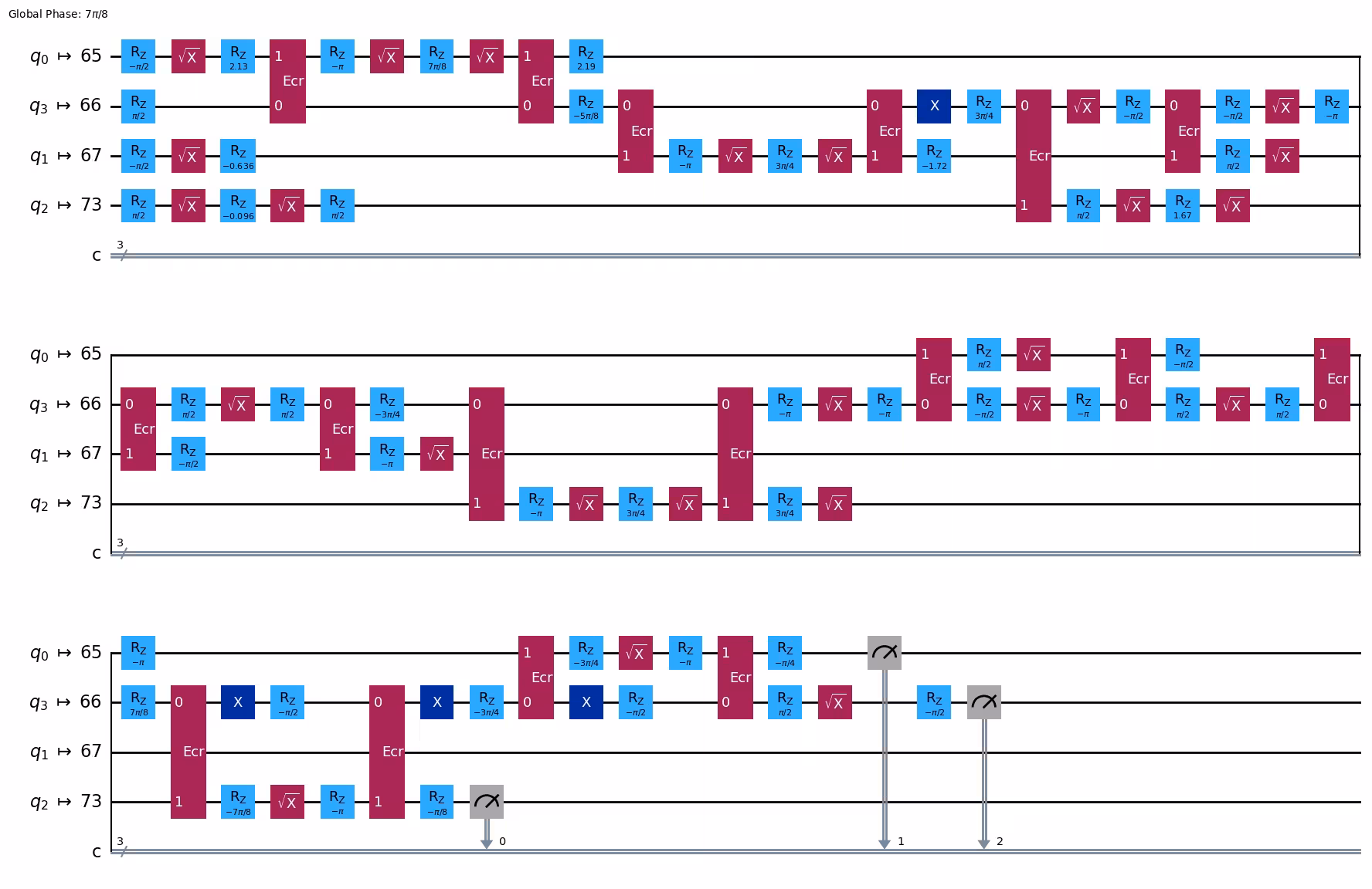
4.2 Hakbang 2: I-optimize para sa target na hardware

# Transpile the circuit into basis gates executable on the hardware
pm = generate_preset_pass_manager(backend=backend, optimization_level=2)
qc_compiled = pm.run(qpe)

qc_compiled.draw("mpl", idle_wires=False)

4.3 Hakbang 3: Patakbuhin sa target na hardware

real_sampler = Sampler(mode=backend)
job = real_sampler.run([qc_compiled], shots=1024)
job_id = job.job_id()
print("job id:", job_id)

job id: d13p4zb5z6q00087ag00

job = service.job(job_id)  # Input your job-id between the quotations
job.status()

'DONE'

result_real = job.result()
print(result_real)

PrimitiveResult([SamplerPubResult(data=DataBin(c=BitArray(<shape=(), num_shots=1024, num_bits=3>)), metadata={'circuit_metadata': {}})], metadata={'execution': {'execution_spans': ExecutionSpans([DoubleSliceSpan(<start='2025-06-09 22:39:00', stop='2025-06-09 22:39:00', size=1024>)])}, 'version': 2})

4.4 Hakbang 4: I-post-process ang mga resulta

from qiskit.visualization import plot_histogram

plot_histogram(result_real[0].data.c.get_counts())

# See the version of Qiskit
import qiskit

qiskit.__version__

'2.0.2'