Mga quantum algorithm: Mga variational quantum algorithm

tala

Takashi Imamichi (24 May 2024)

I-download ang pdf ng orihinal na lektura. Tandaan na ang ilang mga code snippet ay maaaring maging deprecated dahil static na mga larawan ang mga ito.

Ang tinatayang oras ng QPU para patakbuhin ang eksperimentong ito ay 9 minuto (nasubok sa isang Eagle processor).

(Maaaring hindi matatapos ang notebook na ito sa loob ng oras na pinahihintulutan ng Open Plan. Pakigamit nang maingat ang mga mapagkukunan ng quantum computing.)

1. Panimula

Ang tutorial na ito ay nagbibigay ng pangkalahatang-ideya ng isang hybrid quantum-classical na algorithm, na nakatuon lalo na sa variational quantum eigensolver (VQE) at sa quantum approximate optimization algorithm (QAOA). Ang pangunahing layunin ng mga algorithm na ito ay harapin ang mga optimization problem sa pamamagitan ng paggamit ng mga quantum circuit na may mga parameterized quantum gate.

Sa kabila ng mga pagsulong sa quantum computing, ang presensya ng ingay sa mga kasalukuyang quantum device ay nagpapahirap na makakuha ng makabuluhang mga resulta mula sa malalim na mga quantum circuit. Upang malampasan ang hamong ito, ang VQE at QAOA ay gumagamit ng hybrid quantum-classical na diskarte, na kinabibilangan ng paulit-ulit na pagpapatakbo ng medyo maiikling quantum circuit gamit ang quantum computation at pag-optimize ng mga parameter ng target na parameterized quantum circuit gamit ang classical computation.

Ang QAOA ay may potensyal na magbigay ng mga pinakamainam na solusyon sa mga target na problema sa antas ng utility, salamat sa paggamit ng iba't ibang teknik ng error mitigation at suppression. Ang VQE naman ay may maraming aplikasyon (tulad ng quantum chemistry) kung saan ito ay hindi gaanong scalable. Ngunit lumabas na ang ilang mga diskarte na nauugnay sa eigenvalue upang umakma at palakasin ang VQE, kabilang ang Krylov subspace diagonalization at sampling-based quantum diagonalization (SQD). Ang pag-unawa sa VQE ay isang mahalagang unang hakbang sa pag-unawa sa malawak na hanay ng mga classical-quantum hybrid algorithm na lumabas na.

Inilalarawan ng modyul na ito ang mga pundamental na konsepto at implementasyon ng VQE at QAOA. Ang mga karagdagang tutorial ay magsasaliksik ng mga advanced na paksa at teknik para sa pag-scale up ng mga algorithm na ito. Kailangan mo ang sumusunod na library sa iyong environment para patakbuhin ang notebook na ito. Kung hindi mo pa ito na-install, maaari mo itong i-install sa pamamagitan ng pag-uncomment at pagpapatakbo ng sumusunod na cell.

# Added by doQumentation — required packages for this notebook
!pip install -q matplotlib numpy qiskit qiskit-ibm-runtime rustworkx scipy

# % pip install 'qiskit[visualization]' qiskit-ibm-runtime

2. Pagkuha ng pinakamababang eigenvalue ng isang simpleng Hamiltonian

Magsisimula tayo sa pamamagitan ng pag-apply ng VQE sa isang napaka-simpleng kaso, para makita kung paano ito gumagana. Kukuha tayo ng pinakamababang eigenvalue ng Pauli $Z$ matrix gamit ang VQE. Magsisimula tayo sa pag-import ng ilang pangkalahatang pakete.

import numpy as np
from qiskit.circuit import ParameterVector, QuantumCircuit
from qiskit.primitives import StatevectorEstimator, StatevectorSampler
from qiskit.quantum_info import SparsePauliOp
from scipy.optimize import minimize

Ngayon ay tinutukuyin natin ang operator na interesado tayo at tinitingnan ito sa matrix form.

op = SparsePauliOp("Z")
op.to_matrix()

array([[ 1.+0.j,  0.+0.j],
       [ 0.+0.j, -1.+0.j]])

Madali itong makuha ang mga eigenvalue nang klasikal, kaya maaari nating suriin ang ating gawa. Maaaring mahirap ito habang nagsc-scale tayo patungo sa utility. Dito ginagamit natin ang numpy.

# compute eigenvalues with numpy
result = np.linalg.eigh(op.to_matrix())
print("Eigenvalues:", result.eigenvalues)

Eigenvalues: [-1.  1.]

Para makuha ang mga eigenvalue gamit ang isang variational quantum algorithm, nagtatayo tayo ng circuit na may mga gate na tumatanggap ng mga variational parameter:

# define a variational form
param = ParameterVector("a", 3)
qc = QuantumCircuit(1, 1)
qc.u(param[0], param[1], param[2], 0)
qc_estimator = qc.copy()
qc.measure(0, 0)
qc.draw("mpl")

Kung gusto nating tantiyahin ang expected value ng isang operator (tulad ng $Z$), dapat gumamit tayo ng Estimator. Kung gusto nating tingnan ang mga estado ng sistema, gumagamit tayo ng Sampler.

sampler = StatevectorSampler()
estimator = StatevectorEstimator()

Maaari tayong makakuha ng mga bilang ng mga bitstring na 0 at 1 na may mga random na parameter value na [1, 2, 3] gamit ang Sampler.

# compute counts of bitstrings with random parameter values by Sampler
result = sampler.run([(qc, [1, 2, 3])]).result()
counts = result[0].data.c.get_counts()
counts

{'0': 783, '1': 241}

Alam natin na maaari nating kalkulahin ang expected value ng Z sa pamamagitan ng $\langle Z \rangle = p_0 - p_1$ na may mga probabilidad na $\{0: p_0, 1: p_1\}$.

# compute the expectation value of Z based on the counts
(counts.get("0", 0) - counts.get("1", 0)) / sum(counts.values())

0.529296875

Gumana ang circuit na ito, ngunit ang mga piniling parameter value ay hindi naaayon sa isang estado na may napakababang enerhiya (o mababang eigenvalue). Ang nakuhang eigenvalue ay medyo mas mataas kaysa sa pinakamababa. Katulad ang resulta kapag ginagamit ang estimator.

Tandaan na ang Estimator ay tumatanggap ng mga quantum circuit na walang mga measurement.

result = estimator.run([(qc_estimator, op, [1, 2, 3])]).result()
result[0].data.evs

array(0.54030231)

Kakailanganin nating maghanap sa mga parameter at hanapin ang mga nagbibigay ng pinakamababang eigenvalue. Gumagawa tayo ng function upang makatanggap ng mga parameter value ng variational form at ibalik ang expected value na $\langle Z \rangle$.

# define a cost function to look for the minimum eigenvalue of Z
def cost(x):
    result = sampler.run([(qc, x)]).result()
    counts = result[0].data.c.get_counts()
    expval = (counts.get("0", 0) - counts.get("1", 0)) / sum(counts.values())
    # the following line shows the trajectory of the optimization
    print(expval, counts)
    return expval

Gamitin natin ang minimize function ng SciPy para hanapin ang pinakamababang eigenvalue ng Z.

# minimize the cost function with scipy's minimize
min_result = minimize(cost, [0, 0, 0], method="COBYLA", tol=1e-8)
min_result

1.0 {'0': 1024}
0.494140625 {'0': 765, '1': 259}
0.466796875 {'0': 751, '1': 273}
0.564453125 {'0': 801, '1': 223}
-0.4296875 {'1': 732, '0': 292}
-0.984375 {'1': 1016, '0': 8}
-0.8984375 {'1': 972, '0': 52}
-0.990234375 {'1': 1019, '0': 5}
-0.892578125 {'1': 969, '0': 55}
-0.986328125 {'1': 1017, '0': 7}
-0.861328125 {'1': 953, '0': 71}
-1.0 {'1': 1024}
-0.982421875 {'1': 1015, '0': 9}
-0.99609375 {'1': 1022, '0': 2}
-0.986328125 {'1': 1017, '0': 7}
-1.0 {'1': 1024}
-0.990234375 {'1': 1019, '0': 5}
-0.998046875 {'1': 1023, '0': 1}
-0.99609375 {'1': 1022, '0': 2}
-1.0 {'1': 1024}
-1.0 {'1': 1024}
-1.0 {'1': 1024}
-1.0 {'1': 1024}
-0.998046875 {'1': 1023, '0': 1}
-1.0 {'1': 1024}
-1.0 {'1': 1024}
-0.998046875 {'1': 1023, '0': 1}
-0.998046875 {'1': 1023, '0': 1}
-0.998046875 {'1': 1023, '0': 1}
-1.0 {'1': 1024}
-0.99609375 {'1': 1022, '0': 2}
-1.0 {'1': 1024}
-0.99609375 {'1': 1022, '0': 2}
-0.998046875 {'1': 1023, '0': 1}
-0.998046875 {'1': 1023, '0': 1}
-0.99609375 {'1': 1022, '0': 2}
-0.998046875 {'1': 1023, '0': 1}
-1.0 {'1': 1024}
-0.998046875 {'1': 1023, '0': 1}
-0.998046875 {'1': 1023, '0': 1}
-0.99609375 {'1': 1022, '0': 2}
-1.0 {'1': 1024}
-0.998046875 {'1': 1023, '0': 1}
-1.0 {'1': 1024}
-0.998046875 {'1': 1023, '0': 1}
-0.998046875 {'1': 1023, '0': 1}
-1.0 {'1': 1024}
-0.998046875 {'1': 1023, '0': 1}
-0.998046875 {'1': 1023, '0': 1}
-1.0 {'1': 1024}
-1.0 {'1': 1024}
-1.0 {'1': 1024}
-1.0 {'1': 1024}
-1.0 {'1': 1024}
-1.0 {'1': 1024}
-0.998046875 {'1': 1023, '0': 1}
-0.994140625 {'1': 1021, '0': 3}
-1.0 {'1': 1024}
-1.0 {'1': 1024}
-1.0 {'1': 1024}
-1.0 {'1': 1024}
-1.0 {'1': 1024}
-1.0 {'1': 1024}

message: Optimization terminated successfully.
 success: True
  status: 1
     fun: -1.0
       x: [ 3.182e+00  1.338e+00  1.664e-01]
    nfev: 63
   maxcv: 0.0

# check counts of bitstrings with the optimal parameters
result = sampler.run([(qc, min_result.x)]).result()
result[0].data.c.get_counts()

{'0': 1, '1': 1023}

2.1 Ehersisyo

Kalkulahin ang pinakamababang eigenvalue ng $Z \otimes Z$ gamit ang VQE.

z2 = SparsePauliOp("ZZ")
print(z2)
print(z2.to_matrix())

SparsePauliOp(['ZZ'],
              coeffs=[1.+0.j])
[[ 1.+0.j  0.+0.j  0.+0.j  0.+0.j]
 [ 0.+0.j -1.+0.j  0.+0.j  0.+0.j]
 [ 0.+0.j  0.+0.j -1.+0.j  0.+0.j]
 [ 0.+0.j  0.+0.j  0.+0.j  1.+0.j]]

# compute eigenvalues with numpy

# define a variational form
# qc = ...

# compute counts of bitstrings with a random parameter values by Sampler
# result = sampler.run(...)
# result

# compute the expectation value of ZZ based on the counts

# verify the expectation value of ZZ with Estimator

# define a cost function to look for the minimum eigenvalue of ZZ
# def cost(x):
#    expval = ...
#    return expval

# minimize the cost function with scipy's minimize
# min_result = minimize(cost, [...], method="COBYLA", tol=1e-8)
# min_result

# check counts of bitstrings with the optimal parameter values
# result = sampler.run(qc, min_result.x).result()
# result

Mga solusyon sa ehersisyo

Tinutukuyin natin ang operator na interesado tayo at tinitingnan ito sa matrix form.

z2 = SparsePauliOp("ZZ")
print(z2)
print(z2.to_matrix())

SparsePauliOp(['ZZ'],
              coeffs=[1.+0.j])
[[ 1.+0.j  0.+0.j  0.+0.j  0.+0.j]
 [ 0.+0.j -1.+0.j  0.+0.j  0.+0.j]
 [ 0.+0.j  0.+0.j -1.+0.j  0.+0.j]
 [ 0.+0.j  0.+0.j  0.+0.j  1.+0.j]]

Para makuha ang mga eigenvalue gamit ang isang variational quantum algorithm, nagtatayo tayo ng circuit na may mga gate na tumatanggap ng mga variational parameter:

# define a variational form
param = ParameterVector("a", 6)
qc = QuantumCircuit(2, 2)
qc.u(param[0], param[1], param[2], 0)
qc.u(param[3], param[4], param[5], 1)
qc_estimator = qc.copy()
qc.measure([0, 1], [0, 1])
qc.draw("mpl")

Kung gusto nating tantiyahin ang expected value ng isang operator (tulad ng $Z \otimes Z$), gagamit tayo ng Estimator. Kung gusto nating tingnan ang mga estado ng sistema, gumagamit tayo ng Sampler.

sampler = StatevectorSampler()
estimator = StatevectorEstimator()

# compute counts of bitstrings with random parameter values by Sampler
result = sampler.run([(qc, [1, 2, 3, 4, 5, 6])]).result()
counts = result[0].data.c.get_counts()
counts

{'10': 661, '11': 203, '01': 47, '00': 113}

# compute the expectation value of ZZ based on the counts
(
    counts.get("00", 0)
    - counts.get("01", 0)
    - counts.get("10", 0)
    + counts.get("11", 0)
) / sum(counts.values())

-0.3828125

Gumana ang circuit na ito, ngunit ang mga piniling parameter value ay hindi naaayon sa isang estado na may napakababang enerhiya (o mababang eigenvalue). Ang nakuhang eigenvalue ay medyo mas mataas kaysa sa pinakamababa. Katulad ang resulta kapag ginagamit ang estimator.

# verify the expectation value of ZZ with Estimator
result = estimator.run([(qc_estimator, z2, [1, 2, 3, 4, 5, 6])]).result()
result[0].data.evs

array(-0.35316516)

Kakailanganin nating maghanap sa mga parameter at hanapin ang mga nagbibigay ng pinakamababang eigenvalue.

# define a cost function to look for the minimum eigenvalue of ZZ
def cost(x):
    result = sampler.run([(qc, x)]).result()
    counts = result[0].data.c.get_counts()
    expval = (
        counts.get("00", 0)
        - counts.get("01", 0)
        - counts.get("10", 0)
        + counts.get("11", 0)
    ) / sum(counts.values())
    print(expval, counts)
    return expval

# minimize the cost function with scipy's minimize
min_result = minimize(cost, [0, 0, 0, 0, 0, 0], method="COBYLA", tol=1e-8)
min_result

1.0 {'00': 1024}
0.578125 {'00': 808, '01': 216}
0.5234375 {'00': 780, '01': 244}
0.548828125 {'00': 793, '01': 231}
0.3515625 {'00': 637, '10': 164, '11': 55, '01': 168}
0.3359375 {'00': 638, '11': 46, '10': 174, '01': 166}
0.283203125 {'00': 602, '10': 181, '01': 186, '11': 55}
-0.087890625 {'01': 414, '00': 184, '10': 143, '11': 283}
0.236328125 {'10': 27, '11': 623, '01': 364, '00': 10}
-0.0625 {'11': 261, '01': 403, '00': 219, '10': 141}
0.248046875 {'01': 366, '11': 628, '00': 11, '10': 19}
-0.0625 {'10': 145, '11': 254, '01': 399, '00': 226}
0.228515625 {'01': 373, '11': 609, '00': 20, '10': 22}
0.0546875 {'11': 376, '10': 273, '01': 211, '00': 164}
-0.447265625 {'01': 731, '10': 10, '11': 267, '00': 16}
-0.71484375 {'01': 871, '11': 99, '00': 47, '10': 7}
-0.46484375 {'01': 741, '00': 253, '10': 9, '11': 21}
-0.87890625 {'01': 962, '00': 39, '11': 23}
-0.640625 {'00': 176, '01': 837, '11': 8, '10': 3}
-0.88671875 {'01': 966, '00': 41, '11': 17}
-0.994140625 {'01': 1021, '11': 3}
-0.91796875 {'01': 982, '11': 35, '00': 7}
-0.994140625 {'01': 1021, '11': 2, '00': 1}
-0.939453125 {'01': 993, '00': 31}
-0.990234375 {'01': 1019, '11': 5}
-0.90234375 {'01': 974, '00': 21, '11': 29}
-0.98046875 {'01': 1014, '11': 10}
-0.994140625 {'01': 1021, '00': 3}
-0.990234375 {'01': 1019, '11': 4, '00': 1}
-0.98828125 {'01': 1018, '11': 6}
-0.990234375 {'01': 1019, '11': 4, '00': 1}
-0.994140625 {'01': 1021, '11': 2, '00': 1}
-0.99609375 {'01': 1022, '11': 2}
-0.998046875 {'01': 1023, '00': 1}
-0.99609375 {'01': 1022, '00': 2}
-1.0 {'01': 1024}
-1.0 {'01': 1024}
-1.0 {'01': 1024}
-0.998046875 {'01': 1023, '11': 1}
-1.0 {'01': 1024}
-1.0 {'01': 1024}
-1.0 {'01': 1024}
-1.0 {'01': 1024}
-1.0 {'01': 1024}
-1.0 {'01': 1024}
-1.0 {'01': 1024}
-0.998046875 {'01': 1023, '00': 1}
-0.998046875 {'01': 1023, '11': 1}
-0.998046875 {'01': 1023, '00': 1}
-1.0 {'01': 1024}
-1.0 {'01': 1024}
-1.0 {'01': 1024}
-1.0 {'01': 1024}
-1.0 {'01': 1024}
-1.0 {'01': 1024}
-0.998046875 {'01': 1023, '11': 1}
-0.998046875 {'01': 1023, '11': 1}
-1.0 {'01': 1024}
-1.0 {'01': 1024}
-0.998046875 {'01': 1023, '11': 1}
-0.998046875 {'01': 1023, '11': 1}
-0.998046875 {'01': 1023, '00': 1}
-1.0 {'01': 1024}
-1.0 {'01': 1024}
-0.998046875 {'01': 1023, '00': 1}
-1.0 {'01': 1024}
-1.0 {'01': 1024}
-1.0 {'01': 1024}
-1.0 {'01': 1024}
-0.998046875 {'01': 1023, '11': 1}
-0.998046875 {'01': 1023, '11': 1}
-1.0 {'01': 1024}
-0.998046875 {'01': 1023, '11': 1}
-1.0 {'01': 1024}
-1.0 {'01': 1024}
-1.0 {'01': 1024}
-0.998046875 {'01': 1023, '11': 1}
-0.998046875 {'01': 1023, '11': 1}
-1.0 {'01': 1024}
-1.0 {'01': 1024}
-0.998046875 {'01': 1023, '11': 1}
-0.998046875 {'01': 1023, '11': 1}
-0.998046875 {'01': 1023, '00': 1}
-1.0 {'01': 1024}
-1.0 {'01': 1024}
-1.0 {'01': 1024}
-0.998046875 {'01': 1023, '11': 1}
-1.0 {'01': 1024}
-0.99609375 {'01': 1022, '00': 1, '11': 1}
-0.998046875 {'01': 1023, '11': 1}
-0.998046875 {'01': 1023, '00': 1}
-0.998046875 {'01': 1023, '11': 1}
-1.0 {'01': 1024}
-0.99609375 {'01': 1022, '11': 1, '00': 1}
-1.0 {'01': 1024}
-0.998046875 {'01': 1023, '00': 1}
-0.994140625 {'01': 1021, '00': 3}
-0.998046875 {'01': 1023, '00': 1}
-0.99609375 {'01': 1022, '11': 2}
-1.0 {'01': 1024}
-1.0 {'01': 1024}
-0.998046875 {'01': 1023, '11': 1}
-1.0 {'01': 1024}
-1.0 {'01': 1024}
-1.0 {'01': 1024}
-1.0 {'01': 1024}
-1.0 {'01': 1024}
-1.0 {'01': 1024}
-0.998046875 {'01': 1023, '11': 1}
-1.0 {'01': 1024}
-1.0 {'01': 1024}
-1.0 {'01': 1024}
-0.998046875 {'01': 1023, '11': 1}
-0.998046875 {'01': 1023, '11': 1}
-1.0 {'01': 1024}
-0.998046875 {'01': 1023, '00': 1}
-1.0 {'01': 1024}
-1.0 {'01': 1024}
-1.0 {'01': 1024}
-1.0 {'01': 1024}
-1.0 {'01': 1024}
-1.0 {'01': 1024}
-0.998046875 {'01': 1023, '11': 1}
-0.998046875 {'01': 1023, '11': 1}
-0.998046875 {'01': 1023, '11': 1}
-0.99609375 {'01': 1022, '11': 2}
-1.0 {'01': 1024}
-0.998046875 {'01': 1023, '11': 1}

message: Optimization terminated successfully.
 success: True
  status: 1
     fun: -0.998046875
       x: [ 3.167e+00  6.940e-01  1.033e+00 -2.894e-02  8.933e-01
            1.885e+00]
    nfev: 128
   maxcv: 0.0

message: Optimization terminated successfully.
 success: True
  status: 1
     fun: -0.99609375
       x: [ 3.098e+00 -5.402e-01  1.091e+00 -1.004e-02  3.615e-01
            6.913e-01]
    nfev: 115
   maxcv: 0.0

Nakakuha tayo ng eigenvalue na napakalapit sa pinakamababa na ibinigay sa atin ng numpy.

# check counts of bitstrings with the optimal parameters
result = sampler.run([(qc, min_result.x)]).result()
result[0].data.c.get_counts()

{'01': 1024}

3. Quantum Optimization gamit ang Qiskit Patterns

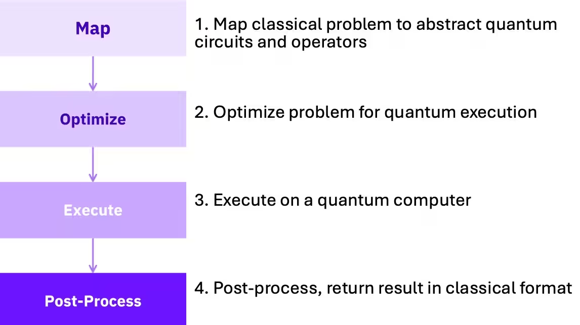
Sa how-to na ito, matututunan natin ang tungkol sa Qiskit patterns at quantum approximate optimization. Ang Qiskit pattern ay isang intuitive at paulit-ulit na hanay ng mga hakbang para sa pagpapatupad ng quantum computing workflow: Ilalapat natin ang mga pattern sa konteksto ng combinatorial optimization at ipapakita kung paano solusyunan ang problemang Max-Cut gamit ang Quantum Approximate Optimization Algorithm (QAOA), isang hybrid (quantum-classical) na iterative na pamamaraan.

Tandaan na ang bahaging QAOA na ito ay batay sa "Part 1: Small-scale QAOA" ng tutorial na Quantum approximate optimization algorithm. Tingnan ang tutorial para matutunan kung paano ito palawakin.

3.1 (Small-scale) Qiskit Pattern para sa Optimization

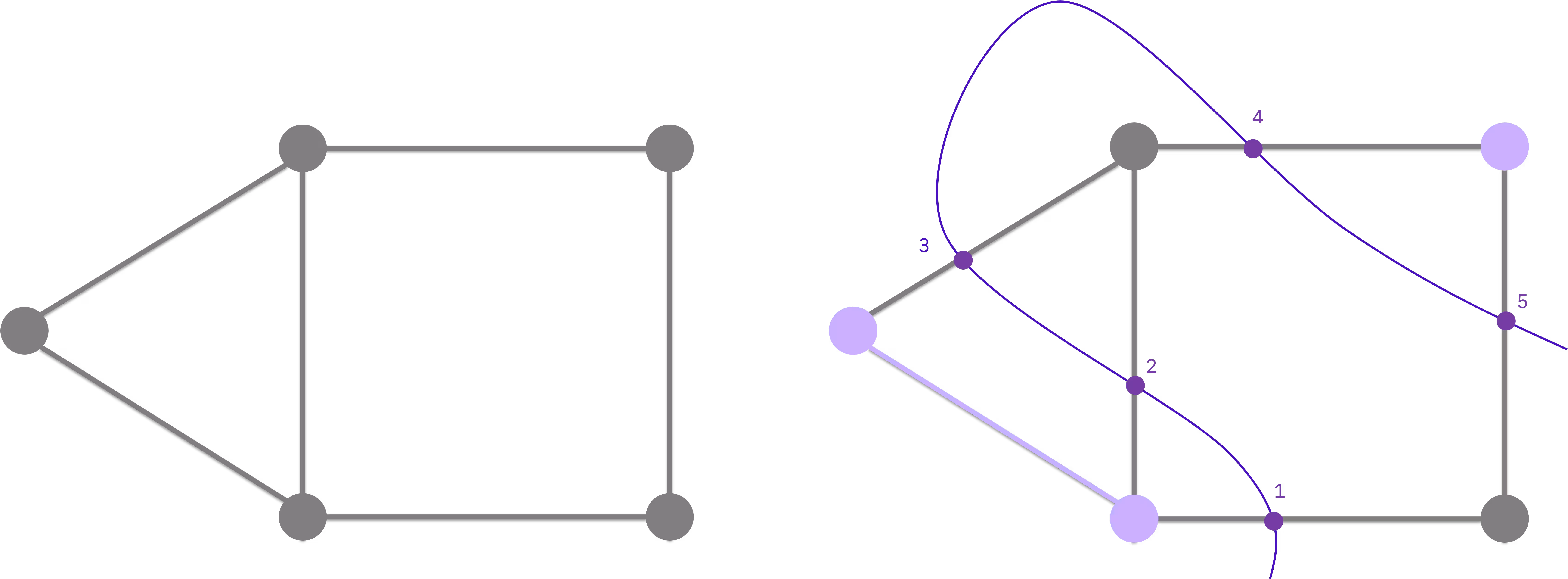
Gagamitin ng bahaging ito ang isang maliit na Max-Cut na problema para ilarawan ang mga hakbang na kailangan para malutas ang isang optimization problem gamit ang quantum computer. Ang Max-Cut na problema ay isang optimization problem na mahirap solusyunan (mas tiyak, isa itong NP-hard na problema) na may iba't ibang aplikasyon sa clustering, network science, at statistical physics. Isinasaalang-alang ng tutorial na ito ang isang graph ng mga node na konektado ng mga edge at layunin nitong hatiin ang mga node sa dalawang grupo sa pamamagitan ng "pagputol" ng mga edge, upang mapakinabangan ang bilang ng mga edge na naaputol. Para magbigay ng konteksto bago i-map ang problemang ito sa isang quantum algorithm, mas mauunawaan mo kung paano nagiging classical combinatorial optimization problem ang Max-Cut sa pamamagitan ng pagsasaalang-alang muna ng minimization ng isang function na $f(x)$

$$\min_{x\in \{0, 1\}^n}f(x),$$

kung saan ang input na $x$ ay isang vector na ang mga bahagi ay naaayon sa bawat node ng isang graph. Pagkatapos, pigilan ang bawat bahagi na maging alinman sa $0$ o $1$ (na kumakatawan sa pagiging kasama o hindi kasama sa cut). Ang maliit na halimbawang ito ay gumagamit ng graph na may $n=5$ na node.

Maaari kang sumulat ng function para sa isang pares ng mga node na $i,j$ na nagpapahiwatig kung ang kaukulang edge na $(i,j)$ ay nasa cut. Halimbawa, ang function na $x_i + x_j - 2 x_i x_j$ ay 1 lamang kung isa sa $x_i$ o $x_j$ ay 1 (na nangangahulugang ang edge ay nasa cut) at zero kung hindi. Ang problema ng pagpapakinabang ng mga edge sa cut ay maaaring buuin bilang

$$\max_{x\in \{0, 1\}^n} \sum_{(i,j)} x_i + x_j - 2 x_i x_j,$$

na maaaring isulat muli bilang isang minimization na may anyo

$$\min_{x\in \{0, 1\}^n} \sum_{(i,j)} 2 x_i x_j - x_i - x_j.$$

Ang minimum ng $f(x)$ sa kasong ito ay kapag ang bilang ng mga edge na tinatagos ng cut ay pinakamataas. Tulad ng nakikita mo, wala pang kaugnayan sa quantum computing. Kailangan mong baguhin ang formulasyon ng problemang ito sa isang bagay na mauunawaan ng quantum computer. Simulan ang iyong problema sa pamamagitan ng paglikha ng graph na may $n=5$ na node.

import matplotlib
import matplotlib.pyplot as plt
import numpy as np
import rustworkx as rx
from rustworkx.visualization import mpl_draw

n = 5

graph = rx.PyGraph()
graph.add_nodes_from(range(1, n + 1))
edge_list = [
    (0, 1, 1.0),
    (0, 2, 1.0),
    (1, 2, 1.0),
    (1, 3, 1.0),
    (2, 4, 1.0),
    (3, 4, 1.0),
]
graph.add_edges_from(edge_list)
pos = rx.spring_layout(graph, seed=2)
mpl_draw(graph, node_size=600, pos=pos, with_labels=True, labels=str)

3.2 Hakbang 1. I-map ang mga Classical Input sa isang Quantum Problem

Ang unang hakbang ng pattern ay ang pag-map ng classical na problema (graph) sa mga quantum circuit at operator. Para magawa ito, may tatlong pangunahing hakbang na dapat sundin:

1. Gumamit ng serye ng mga mathematical reformulation para katawanin ang problemang ito gamit ang notasyon ng Quadratic Unconstrained Binary Optimization (QUBO).
2. Isulat muli ang optimization problem bilang isang Hamiltonian na ang ground state ay naaayon sa solusyon na nagpapababa ng cost function.
3. Lumikha ng quantum circuit na maghahanda ng ground state ng Hamiltoniang ito sa pamamagitan ng isang prosesong katulad ng quantum annealing.

Tandaan: Sa metodolohiya ng QAOA, ang layunin mo sa huli ay magkaroon ng isang operator (Hamiltonian) na kumakatawan sa cost function ng ating hybrid algorithm, pati na rin ang isang parametrized circuit (Ansatz) na kumakatawan sa mga quantum state na may mga candidate na solusyon sa problema. Maaari kang mag-sample mula sa mga candidate na state na ito at pagkatapos ay suriin ang mga ito gamit ang cost function.

Graph → optimization problem

Ang unang hakbang ng mapping ay isang pagbabago ng notasyon. Ang sumusunod ay nagpapahayag ng problema sa QUBO notation:

$$\min_{x\in \{0, 1\}^n}x^T Q x,$$

kung saan ang $Q$ ay isang $n\times n$ na matrix ng mga tunay na numero, ang $n$ ay naaayon sa bilang ng mga node sa iyong graph, ang $x$ ay ang vector ng mga binary variable na ipinakilala sa itaas, at ang $x^T$ ay nagpapahiwatig ng transpose ng vector na $x$.

Problem name: maxcut

Minimize
  2*x_1*x_2 + 2*x_1*x_3 + 2*x_2*x_3 + 2*x_2*x_4 + 2*x_3*x_5 + 2*x_4*x_5 - 2*x_1
  - 3*x_2 - 3*x_3 - 2*x_4 - 2*x_5

Subject to
  No constraints

  Binary variables (5)
    x_1 x_2 x_3 x_4 x_5

Optimization problem → Hamiltonian

Maaari mo ring baguhin ang formulasyon ng QUBO problem bilang isang Hamiltonian (dito, isang matrix na kumakatawan sa enerhiya ng isang sistema):

$$H_C=\sum_{ij}Q_{ij}Z_iZ_j + \sum_i b_iZ_i.$$

Mga hakbang ng reformulation mula sa QAOA problem patungong Hamiltonian

Para ipakita kung paano maisusulat muli ang QAOA problem sa ganitong paraan, palitan muna ang mga binary variable na $x_i$ ng isang bagong hanay ng mga variable na $z_i\in\{-1, 1\}$ sa pamamagitan ng

$$x_i = \frac{1-z_i}{2}.$$

Makikita dito na kung ang $x_i$ ay $0$, ang $z_i$ ay dapat na $1$. Kapag pinalitan ang mga $x_i$ ng $z_i$ sa optimization problem ($x^TQx$), maaaring makuha ang isang katumbas na formulasyon.

$$x^TQx=\sum_{ij}Q_{ij}x_ix_j \\ =\frac{1}{4}\sum_{ij}Q_{ij}(1-z_i)(1-z_j) \\=\frac{1}{4}\sum_{ij}Q_{ij}z_iz_j-\frac{1}{4}\sum_{ij}(Q_{ij}+Q_{ji})z_i + \frac{n^2}{4}.$$

Ngayon kung tukuyin natin ang $b_i=-\sum_{j}(Q_{ij}+Q_{ji})$, alisin ang prefactor, at ang constant na $n^2$ na term, maaabot natin ang dalawang katumbas na formulasyon ng parehong optimization problem.

$$min_{x\in\{0,1\}^n} x^TQx\Longleftrightarrow \min_{z\in\{-1,1\}^n}z^TQz + b^Tz$$

Dito, ang $b$ ay nakasalalay sa $Q$. Tandaan na para makuha ang $z^TQz + b^Tz$ inalis natin ang factor na 1/4 at isang constant offset na $n^2$ na hindi gumaganap ng papel sa optimization.

Ngayon, para makuha ang quantum formulation ng problema, i-promote ang mga variable na $z_i$ sa isang Pauli $Z$ matrix, tulad ng isang $2\times 2$ na matrix na may anyo

$$Z_i = \begin{pmatrix}1 & 0 \\ 0 & -1\end{pmatrix}.$$

Kapag pinalitan mo ang mga matrix na ito sa optimization problem sa itaas, makukuha mo ang sumusunod na Hamiltonian

$$H_C=\sum_{ij}Q_{ij}Z_iZ_j + \sum_i b_iZ_i.$$

Tandaan din na ang mga $Z$ matrix ay naka-embed sa computational space ng quantum computer, iyon ay, isang Hilbert space na may sukat na $2^n\times 2^n$. Samakatuwid, dapat maunawaan ang mga term tulad ng $Z_iZ_j$ bilang ang tensor product na $Z_i\otimes Z_j$ na naka-embed sa $2^n\times 2^n$ na Hilbert space. Halimbawa, sa isang problema na may limang decision variable, ang term na $Z_1Z_3$ ay nangangahulugang $I\otimes Z_3\otimes I\otimes Z_1\otimes I$ kung saan ang $I$ ay ang $2\times 2$ na identity matrix.

Ang Hamiltonianing ito ay tinatawag na cost function Hamiltonian. Mayroon itong katangian na ang ground state nito ay naaayon sa solusyon na nagpapababa ng cost function na $f(x)$. Samakatuwid, para malutas ang iyong optimization problem kailangan mo na ngayong ihanda ang ground state ng $H_C$ (o isang state na may mataas na overlap nito) sa quantum computer. Pagkatapos, ang pag-sample mula sa state na ito ay magbibigay, na may mataas na posibilidad, ng solusyon sa $\min~f(x)$.

def build_max_cut_operator(graph: rx.PyGraph) -> tuple[SparsePauliOp, float]:
    sp_list = []
    constant = 0
    for s, t in graph.edge_list():
        w = graph.get_edge_data(s, t)
        sp_list.append(("ZZ", [s, t], w / 2))
        constant -= 1 / 2
    return SparsePauliOp.from_sparse_list(
        sp_list, num_qubits=graph.num_nodes()
    ), constant

cost_hamiltonian, constant = build_max_cut_operator(graph)
print("Cost Function Hamiltonian:", cost_hamiltonian)
print("Constant:", constant)

Cost Function Hamiltonian: SparsePauliOp(['IIIZZ', 'IIZIZ', 'IIZZI', 'IZIZI', 'ZIZII', 'ZZIII'],
              coeffs=[0.5+0.j, 0.5+0.j, 0.5+0.j, 0.5+0.j, 0.5+0.j, 0.5+0.j])
Constant: -3.0

Hamiltonian → quantum circuit

Ang Hamiltonian na $H_C$ ay naglalaman ng quantum na kahulugan ng iyong problema. Ngayon ay maaari kang lumikha ng quantum circuit na tutulong sa pag-sample ng magagandang solusyon mula sa quantum computer. Ang QAOA ay inspirado ng quantum annealing at nag-aapply ng mga alternating layer ng mga operator sa quantum circuit.

Ang pangkalahatang ideya ay magsimula sa ground state ng isang kilalang sistema, $H^{\otimes n}|0\rangle$ sa itaas, at pagkatapos ay gabayan ang sistema patungo sa ground state ng cost operator na interesado ka. Ginagawa ito sa pamamagitan ng pag-apply ng mga operator na $\exp\{-i\gamma_k H_C\}$ at $\exp\{-i\beta_k H_m\}$ na may mga anggulo na $\gamma_1,...,\gamma_p$ at $\beta_1,...,\beta_p~$.

Ang quantum circuit na iyong ginagawa ay parametrized ng $\gamma_i$ at $\beta_i$, kaya maaari kang subukan ang iba't ibang halaga ng $\gamma_i$ at $\beta_i$ at mag-sample mula sa resultang state. Sa kasong ito, susubukan natin ang isang halimbawa na may 1 QAOA layer na naglalaman ng dalawang parameter: $\gamma_1$ at $\beta_1$.

from qiskit.circuit.library import QAOAAnsatz

circuit = QAOAAnsatz(cost_operator=cost_hamiltonian, reps=1)
circuit.measure_all()
circuit.draw("mpl")

circuit.decompose(reps=3).draw("mpl", fold=-1)

circuit.parameters

ParameterView([ParameterVectorElement(β[0]), ParameterVectorElement(γ[0])])

3.3 Hakbang 2. I-optimize ang mga circuit para sa Pagsasagawa sa Quantum Hardware

Ang circuit sa itaas ay naglalaman ng serye ng mga abstraksiyon na kapaki-pakinabang para mag-isip tungkol sa mga quantum algorithm, ngunit hindi posibleng patakbuhin sa hardware. Para makapagpatakbo sa isang QPU, ang circuit ay kailangang dumaan sa isang serye ng mga operasyon na bumubuo sa hakbang ng transpilation o circuit optimization ng pattern.

Ang Qiskit library ay nag-aalok ng serye ng mga transpilation pass na nag-aakma sa malawak na hanay ng mga circuit transformation. Kailangan mong tiyakin na ang iyong circuit ay na-optimize para sa iyong layunin.

Ang transpilation ay maaaring magsangkot ng ilang hakbang, tulad ng:

• Initial mapping ng mga qubit sa circuit (tulad ng mga decision variable) sa mga pisikal na qubit sa device.
• Unrolling ng mga instruksyon sa quantum circuit patungo sa mga hardware-native na instruksyon na naiintindihan ng backend.
• Routing ng mga qubit sa circuit na nakikipag-ugnayan sa mga pisikal na qubit na magkakatabi.
• Error suppression sa pamamagitan ng pagdaragdag ng mga single-qubit gate para pigilin ang ingay gamit ang dynamical decoupling.

Ang karagdagang impormasyon tungkol sa transpilation ay makukuha sa aming dokumentasyon.

Ang sumusunod na code ay nag-transform at nag-optimize ng abstract circuit sa isang format na handa na para sa pagpapatupad sa isa sa mga device na accessible sa pamamagitan ng cloud gamit ang Qiskit IBM® Runtime service.

Tandaan na maaari mong subukan ang iyong mga programa nang lokal sa pamamagitan ng "local testing mode" bago ipadala ang mga ito sa mga tunay na quantum computer. Ang karagdagang impormasyon tungkol sa local testing mode ay makukuha sa dokumentasyon.

from qiskit_ibm_runtime import QiskitRuntimeService
from qiskit.transpiler.preset_passmanagers import generate_preset_pass_manager

# Use a quantum device
service = QiskitRuntimeService()
backend = service.least_busy(min_num_qubits=127)
# backend = service.backend("ibm_kingston")

# You can test your programs locally with a fake backend (local testing mode)
# backend = FakeBrisbane()

print(backend)

# Create pass manager for transpilation
pm = generate_preset_pass_manager(optimization_level=3, backend=backend)

candidate_circuit = pm.run(circuit)
candidate_circuit.draw("mpl", fold=False, idle_wires=False)

service = QiskitRuntimeService(channel="ibm_quantum_platform")

<IBMBackend('ibm_strasbourg')>

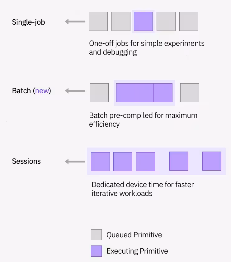
3.4 Hakbang 3. Isagawa gamit ang Qiskit Primitives

Sa QAOA workflow, ang mga optimal na QAOA parameter ay natutuklasan sa pamamagitan ng isang iterative optimization loop, na nagpapatakbo ng serye ng mga circuit evaluation at gumagamit ng classical optimizer para mahanap ang mga optimal na parameter na $\beta_k$ at $\gamma_k$. Ang execution loop na ito ay isinasagawa sa pamamagitan ng mga sumusunod na hakbang:

1. Tukuyin ang mga paunang parameter
2. Mag-instantiate ng bagong Session na naglalaman ng optimization loop at ng primitive na ginagamit para mag-sample ng circuit
3. Kapag natagpuan na ang isang optimal na hanay ng mga parameter, isagawa ang circuit nang isang huling beses para makakuha ng isang panghuling distribusyon na gagamitin sa post-process na hakbang.

Tukuyin ang circuit na may mga paunang parameter

Magsisimula tayo sa mga arbitraryong napiling parameter.

initial_gamma = np.pi
initial_beta = np.pi / 2
init_params = [initial_gamma, initial_beta]

Tukuyin ang backend at execution primitive

Gamitin ang Qiskit Runtime primitives para makipag-ugnayan sa mga IBM® backend. Ang dalawang primitive ay ang Sampler at Estimator, at ang pagpili ng primitive ay nakasalalay sa uri ng sukat na nais mong patakbuhin sa quantum computer. Para sa minimization ng $H_C$, gamitin ang Estimator dahil ang sukat ng cost function ay simpleng expected value ng $\langle H_C \rangle$.

Patakbuhin

Ang mga primitive ay nag-aalok ng iba't ibang execution mode para mag-iskedyul ng mga workload sa mga quantum device, at ang isang QAOA workflow ay tumatakbo nang paulit-ulit sa isang session. Maaari mong ikonekta ang sampler-based na cost function sa SciPy minimizing routine para mahanap ang mga optimal na parameter.

def cost_func_estimator(params, ansatz, hamiltonian, estimator):
    # transform the observable defined on virtual qubits to
    # an observable defined on all physical qubits
    isa_hamiltonian = hamiltonian.apply_layout(ansatz.layout)

    pub = (ansatz, isa_hamiltonian, params)
    job = estimator.run([pub])

    results = job.result()[0]
    cost = results.data.evs

    objective_func_vals.append(cost)

    return cost

from qiskit_ibm_runtime import Session, EstimatorV2
from scipy.optimize import minimize

objective_func_vals = []  # Global variable
with Session(backend=backend) as session:
    # If using qiskit-ibm-runtime<0.24.0, change `mode=` to `session=`
    estimator = EstimatorV2(mode=session)
    estimator.options.default_shots = 1000

    # Set simple error suppression/mitigation options
    estimator.options.dynamical_decoupling.enable = True
    estimator.options.dynamical_decoupling.sequence_type = "XY4"
    estimator.options.twirling.enable_gates = True
    estimator.options.twirling.num_randomizations = "auto"

    result = minimize(
        cost_func_estimator,
        init_params,
        args=(candidate_circuit, cost_hamiltonian, estimator),
        method="COBYLA",
        tol=1e-2,
    )
    print(result)

message: Optimization terminated successfully.
 success: True
  status: 1
     fun: -0.6557925874481715
       x: [ 2.873e+00  9.414e-01]
    nfev: 21
   maxcv: 0.0

Nagawa ng optimizer na bawasan ang cost at makahanap ng mas magagandang parameter para sa circuit.

plt.figure(figsize=(12, 6))
plt.plot(objective_func_vals)
plt.xlabel("Iteration")
plt.ylabel("Cost")
plt.show()

Kapag nahanap mo na ang mga optimal na parameter para sa circuit, maaari mong italaga ang mga parameter na ito at i-sample ang panghuling distribusyon na nakuha gamit ang mga na-optimize na parameter. Dito dapat gamitin ang Sampler primitive dahil ang probability distribution ng mga bitstring measurement ang naaayon sa optimal na cut ng graph.

Tandaan: Nangangahulugan ito ng paghahanda ng quantum state na $\psi$ sa computer at pagkatapos ay pagsusukatan nito. Ang isang sukat ay mag-co-collapse ng state sa isang solong computational basis state — halimbawa, 010101110000... — na naaayon sa isang candidate na solusyon na $x$ sa ating paunang optimization problem ($\max f(x)$ o $\min f(x)$ depende sa gawain).

optimized_circuit = candidate_circuit.assign_parameters(result.x)
optimized_circuit.draw("mpl", fold=False, idle_wires=False)

from qiskit_ibm_runtime import SamplerV2

# If using qiskit-ibm-runtime<0.24.0, change `mode=` to `backend=`
sampler = SamplerV2(mode=backend)

# Set simple error suppression/mitigation options
sampler.options.dynamical_decoupling.enable = True
sampler.options.dynamical_decoupling.sequence_type = "XY4"
sampler.options.twirling.enable_gates = True
sampler.options.twirling.num_randomizations = "auto"

pub = (optimized_circuit,)
job = sampler.run([pub], shots=int(1e4))
counts_int = job.result()[0].data.meas.get_int_counts()
counts_bin = job.result()[0].data.meas.get_counts()
shots = sum(counts_int.values())
final_distribution_int = {key: val / shots for key, val in counts_int.items()}
final_distribution_bin = {key: val / shots for key, val in counts_bin.items()}
print(final_distribution_int)

{12: 0.0652, 31: 0.0089, 4: 0.0085, 13: 0.0731, 26: 0.0256, 28: 0.0246, 17: 0.0405, 25: 0.0591, 20: 0.031, 15: 0.0221, 8: 0.017, 21: 0.0371, 14: 0.0461, 16: 0.0229, 19: 0.0723, 23: 0.0199, 22: 0.0478, 18: 0.0708, 24: 0.0165, 6: 0.0525, 7: 0.0155, 5: 0.0245, 3: 0.0231, 29: 0.0121, 30: 0.0062, 10: 0.0363, 1: 0.0097, 9: 0.042, 27: 0.0094, 11: 0.0349, 0: 0.0129, 2: 0.0119}

3.5 Hakbang 4. Post-process, Ibalik ang Resulta sa Classical Format

Ang post-processing na hakbang ay nagbibigay-kahulugan sa sampling output para ibalik ang isang solusyon para sa iyong orihinal na problema. Sa kasong ito, interesado ka sa bitstring na may pinakamataas na posibilidad dahil ito ang nagtatakda ng optimal na cut. Ang mga simetriya sa problema ay nagbibigay-daan para sa apat na posibleng solusyon, at ang proseso ng pag-sample ay magbabalik ng isa sa mga ito na may bahagyang mas mataas na posibilidad, ngunit makikita sa plotted na distribusyon sa ibaba na apat sa mga bitstring ay kapansin-pansing mas malamang kaysa sa iba.

# auxiliary functions to sample most likely bitstring
def to_bitstring(integer, num_bits):
    result = np.binary_repr(integer, width=num_bits)
    return [int(digit) for digit in result]

keys = list(final_distribution_int.keys())
values = list(final_distribution_int.values())
most_likely = keys[np.argmax(np.abs(values))]
most_likely_bitstring = to_bitstring(most_likely, len(graph))
most_likely_bitstring.reverse()

print("Result bitstring:", most_likely_bitstring)

Result bitstring: [1, 0, 1, 1, 0]

import matplotlib.pyplot as plt

matplotlib.rcParams.update({"font.size": 10})
final_bits = final_distribution_bin
values = np.abs(list(final_bits.values()))
top_4_values = sorted(values, reverse=True)[:4]
positions = []
for value in top_4_values:
    positions.append(np.where(values == value)[0])
fig = plt.figure(figsize=(11, 6))
ax = fig.add_subplot(1, 1, 1)
plt.xticks(rotation=45)
plt.title("Result Distribution")
plt.xlabel("Bitstrings (reversed)")
plt.ylabel("Probability")
ax.bar(list(final_bits.keys()), list(final_bits.values()), color="tab:grey")
for p in positions:
    ax.get_children()[p[0].item()].set_color("tab:purple")
plt.show()

Visualisahin ang pinakamahusay na cut

Mula sa optimal na bit string, maaari mo ring visualisahin ang cut na ito sa orihinal na graph.

colors = ["tab:grey" if i == 0 else "tab:purple" for i in most_likely_bitstring]
mpl_draw(graph, node_size=600, pos=pos, with_labels=True, labels=str, node_color=colors)

At kalkulahin ang halaga ng cut. Ang solusyon ay hindi optimal dahil sa ingay (ang cut value ng optimal na solusyon ay 5).

from typing import Sequence

def evaluate_sample(x: Sequence[int], graph: rx.PyGraph) -> float:
    assert len(x) == len(
        list(graph.nodes())
    ), "The length of x must coincide with the number of nodes in the graph."
    return sum(
        x[u] * (1 - x[v]) + x[v] * (1 - x[u]) for u, v in list(graph.edge_list())
    )

cut_value = evaluate_sample(most_likely_bitstring, graph)
print("The value of the cut is:", cut_value)

The value of the cut is: 5

Tinapos nito ang small-scale QAOA tutorial. Matututunan mo kung paano i-adapt ang QAOA sa utility-scale sa "Part 2: scale it up!" ng tutorial na Quantum approximate optimization algorithm.

# Check Qiskit version
import qiskit

qiskit.__version__

'2.0.2'