Utility-scale na eksperimento III

tala

Toshinari Itoko, Tamiya Onodera, Kifumi Numata (19 Hulyo 2024)

I-download ang pdf ng orihinal na lektura. Tandaan na maaaring maging deprecated na ang ilang code snippet dahil mga static na imahe ang mga ito.

Ang tinatayang oras ng QPU para patakbuhin ang unang eksperimentong ito ay 12 m 30 s. May karagdagang eksperimento sa ibaba na nangangailangan ng humigit-kumulang 4 m.

(Tandaan: maaaring hindi ma-evaluate ang notebook na ito sa loob ng oras na pinapayagan sa Open Plan. Siguraduhing gamitin nang matalino ang mga quantum computing resources.)

# Added by doQumentation — required packages for this notebook
!pip install -q numpy qiskit qiskit-ibm-runtime rustworkx

import qiskit

qiskit.__version__

'2.0.2'

import qiskit_ibm_runtime

qiskit_ibm_runtime.__version__

'0.40.1'

import numpy as np
import rustworkx as rx

from qiskit import QuantumCircuit
from qiskit.visualization import plot_histogram
from qiskit.visualization import plot_gate_map
from qiskit.transpiler.preset_passmanagers import generate_preset_pass_manager
from qiskit.providers import BackendV2
from qiskit.quantum_info import SparsePauliOp

from qiskit_ibm_runtime import QiskitRuntimeService
from qiskit_ibm_runtime import Sampler, Estimator, Batch, SamplerOptions

1. Panimula

Mabilis nating balikan ang GHZ states, at kung anong uri ng distribusyon ang maaari mong asahan mula sa Sampler kapag inilapat dito. Pagkatapos ay malinaw naming ilalatag ang layunin ng araling ito.

1.1 GHZ state

Ang GHZ state (Greenberger-Horne-Zeilinger state) para sa $n$ na qubit ay tinukoy bilang

$$\frac{1}{\sqrt 2}(|0\rangle ^ {\otimes n}+ |1\rangle^ {\otimes n})$$

Natural, maaari itong likhain para sa 6 na qubit gamit ang sumusunod na quantum circuit.

N = 6
qc = QuantumCircuit(N, N)

qc.h(0)
for i in range(N - 1):
    qc.cx(0, i + 1)

# qc.measure_all()
qc.barrier()
qc.measure(list(range(N)), list(range(N)))

qc.draw(output="mpl", idle_wires=False, scale=0.5)

print("Depth:", qc.depth())

Depth: 7

Hindi masyadong malalim ang depth, kahit na alam mo mula sa mga nakaraang aralin na may mas magandang paraan. Pumili tayo ng backend at i-transpile ang circuit na ito.

service = QiskitRuntimeService()
backend = service.least_busy(operational=True, simulator=False)
backend.name
# or
# backend = service.least_busy(operational=True)
# backend.name

'ibm_kingston'

pm = generate_preset_pass_manager(3, backend=backend)
qc_transpiled = pm.run(qc)
qc_transpiled.draw(output="mpl", idle_wires=False, fold=-1)

print("Depth:", qc_transpiled.depth())
print(
    "Two-qubit Depth:",
    qc_transpiled.depth(filter_function=lambda x: x.operation.num_qubits == 2),
)

Depth: 27
Two-qubit Depth: 11

Muli, hindi masyadong malalim ang transpiled two-qubit depth. Ngunit para makipagtulungan sa isang GHZ state na may mas maraming qubit, kailangan mong mag-isip tungkol sa pag-optimize ng circuit. Patakbuhin natin ito gamit ang Sampler at tingnan kung ano ang ibinabalik ng tunay na quantum computer.

sampler = Sampler(mode=backend)
shots = 40000
job = sampler.run([qc_transpiled], shots=shots)
job_id = job.job_id()
print(job_id)

d147y20n2txg008jvv70

job.status()

'DONE'

job = service.job(job_id)
result = job.result()
plot_histogram(result[0].data.c.get_counts(), figsize=(30, 5))

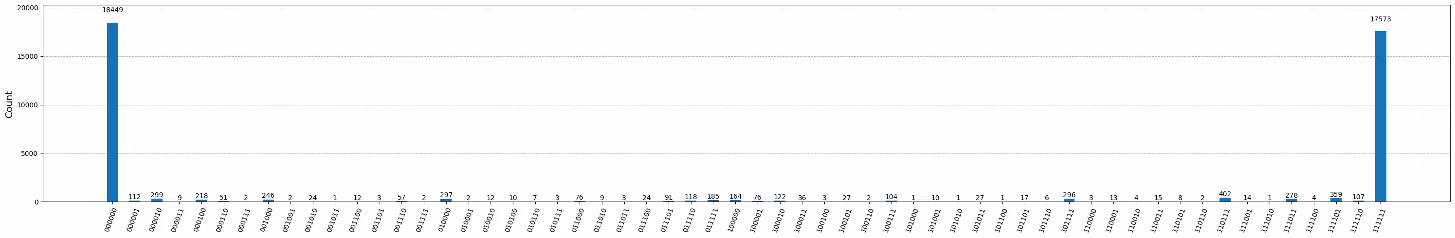
Ito ang resulta ng 6-qubit GHZ circuit. Tulad ng nakikita mo, ang mga estado ng lahat ng $|0\rangle$ at lahat ng $|1\rangle$ ay nangingibabaw nga, ngunit malaki ang mga error. Subukan nating alamin kung gaano kalaki ang GHZ circuit na maaari mong gawin gamit ang isang Eagle device, habang nakakakuha pa rin ng mga resulta kung saan ang mga tamang estado ay may kahit na higit sa 50% na posibilidad.

1.2 Ang iyong layunin

Bumuo ng GHZ circuit para sa 20 qubit o higit pa upang, sa pagsukat, ang fidelity ng iyong GHZ state ay > 0.5. Tandaan:

• Kailangan mong gumamit ng Eagle device (min_num_qubits=127) at itakda ang bilang ng shots bilang 40,000.
• Dapat mong patakbuhin ang GHZ circuit gamit ang function na execute_ghz_fidelity, at kalkulahin ang fidelity gamit ang function na check_ghz_fidelity_from_jobs.

Ito ay inilaan bilang isang independiyenteng ehersisyo, kung saan gagamitin mo ang natutunan mo sa kursong ito hanggang ngayon.

def execute_ghz_fidelity(
    ghz_circuit: QuantumCircuit,  # Quantum circuit to create GHZ state (Circuit after Routing or without Routing), Classical register name is "c"
    physical_qubits: list[int],  # Physical qubits to represent GHZ state
    backend: BackendV2,
    sampler_options: dict | SamplerOptions | None = None,
):
    N_SHOTS = 40_000
    N = len(physical_qubits)
    base_circuit = ghz_circuit.remove_final_measurements(inplace=False)
    # M_k measurement circuits
    mk_circuits = []
    for k in range(1, N + 1):
        circuit = base_circuit.copy()
        # change measurement basis
        for q in physical_qubits:
            circuit.rz(-k * np.pi / N, q)
            circuit.h(q)
        mk_circuits.append(circuit)

    obs = SparsePauliOp.from_sparse_list(
        [("Z" * N, physical_qubits, 1)], num_qubits=backend.num_qubits
    )
    job_ids = []
    pm1 = generate_preset_pass_manager(1, backend=backend)
    org_transpiled = pm1.run(ghz_circuit)
    mk_transpiled = pm1.run(mk_circuits)
    with Batch(backend=backend):
        sampler = Sampler(options=sampler_options)
        sampler.options.twirling.enable_measure = True
        job = sampler.run([org_transpiled], shots=N_SHOTS)
        job_ids.append(job.job_id())
        # print(f"Sampler job id: {job.job_id()}, shots={N_SHOTS}")
        estimator = Estimator()  # TREX is applied as default
        estimator.options.dynamical_decoupling.enable = True
        estimator.options.execution.rep_delay = 0.0005
        estimator.options.twirling.enable_measure = True
        job2 = estimator.run([(circ, obs) for circ in mk_transpiled], precision=1 / 100)
        job_ids.append(job2.job_id())
        # print("Estimator job id:", job2.job_id())
        return [job.job_id(), job2.job_id()]

def check_ghz_fidelity_from_jobs(
    sampler_job,
    estimator_job,
    num_qubits,
    shots=40_000,
):
    N = num_qubits
    sampler_result = sampler_job.result()
    counts = sampler_result[0].data.c.get_counts()
    all_zero = counts.get("0" * N, 0) / shots
    all_one = counts.get("1" * N, 0) / shots
    top3 = sorted(counts, key=counts.get, reverse=True)[:3]
    print(
        f"N={N}: |00..0>: {counts.get('0'*N, 0)}, |11..1>: {counts.get('1'*N, 0)}, |3rd>: {counts.get(top3[2], 0)} ({top3[2]})"
    )
    print(f"P(|00..0>)={all_zero}, P(|11..1>)={all_one}")

    estimator_result = estimator_job.result()
    non_diagonal = (1 / N) * sum(
        (-1) ** k * estimator_result[k - 1].data.evs for k in range(1, N + 1)
    )
    print(f"REM: Coherence (non-diagonal): {non_diagonal:.6f}")
    fidelity = 0.5 * (all_zero + all_one + non_diagonal)
    sigma = 0.5 * np.sqrt(
        (1 - all_zero - all_one) * (all_zero + all_one) / shots
        + sum(estimator_result[k].data.stds ** 2 for k in range(N)) / (N * N)
    )
    print(f"GHZ fidelity = {fidelity:.6f} ± {sigma:.6f}")
    if fidelity - 2 * sigma > 0.5:
        print("GME (genuinely multipartite entangled) test: Passed")
    else:
        print("GME (genuinely multipartite entangled) test: Failed")
    return {
        "fidelity": fidelity,
        "sigma": sigma,
        "shots": shots,
        "job_ids": [sampler_job.job_id(), estimator_job.job_id()],
    }

Sa notebook na ito, maglalapat tayo ng tatlong estratehiya sa paglikha ng magagandang GHZ state gamit ang 16 na qubit at 30 na qubit. Ang mga diskarteng ito ay nadagdag sa mga estratehiya na alam mo na mula sa mga nakaraang aralin.

2. Estratehiya 1. Noise-aware na pagpili ng qubit

Una, tutukuyin natin ang isang backend. Dahil malawak tayong magtatrabaho sa mga katangian ng isang partikular na backend, mainam na tukuyin ang isang backend, kumpara sa paggamit ng opsyong least_busy.

backend = service.backend("ibm_strasbourg")  # eagle
twoq_gate = "ecr"
print(f"Device {backend.name} Loaded with {backend.num_qubits} qubits")
print(f"Two Qubit Gate: {twoq_gate}")

Device ibm_strasbourg Loaded with 127 qubits
Two Qubit Gate: ecr

Magtatayo tayo ng circuit na may maraming two-qubit gate. Makatuwirang gumamit ng mga qubit na may pinakamababang error kapag isinasagawa ang mga two-qubit gate na iyon. Ang paghanap ng pinakamahusay na "qubit chain" batay sa mga iniulat na 2q-gate error ay isang hindi simpleng problema. Ngunit maaari tayong mag-define ng ilang function upang matulungan tayong matukoy kung aling mga qubit ang pinakamainam gamitin.

coupling_map = backend.target.build_coupling_map(twoq_gate)
G = coupling_map.graph

def to_edges(path):  # create edges list from node paths
    edges = []
    prev_node = None
    for node in path:
        if prev_node is not None:
            if G.has_edge(prev_node, node):
                edges.append((prev_node, node))
            else:
                edges.append((node, prev_node))
        prev_node = node
    return edges

def path_fidelity(path, correct_by_duration: bool = True, readout_scale: float = None):
    """Compute an estimate of the total fidelity of 2-qubit gates on a path.
    If `correct_by_duration` is true, each gate fidelity is worsen by
    scale = max_duration / duration, that is, gate_fidelity^scale.
    If `readout_scale` > 0 is supplied, readout_fidelity^readout_scale
    for each qubit on the path is multiplied to the total fielity.
    The path is given in node indices form, for example, [0, 1, 2].
    An external function `to_edges` is used to obtain edge list, for example, [(0, 1), (1, 2)]."""
    path_edges = to_edges(path)
    max_duration = max(backend.target[twoq_gate][qs].duration for qs in path_edges)

    def gate_fidelity(qpair):
        duration = backend.target[twoq_gate][qpair].duration
        scale = max_duration / duration if correct_by_duration else 1.0
        # 1.25 = (d+1)/d with d = 4
        return max(0.25, 1 - (1.25 * backend.target[twoq_gate][qpair].error)) ** scale

    def readout_fidelity(qubit):
        return max(0.25, 1 - backend.target["measure"][(qubit,)].error)

    total_fidelity = np.prod(
        [gate_fidelity(qs) for qs in path_edges]
    )  # two qubits gate fidelity for each path
    if readout_scale:
        total_fidelity *= (
            np.prod([readout_fidelity(q) for q in path]) ** readout_scale
        )  # multiply readout fidelity
    return total_fidelity

def flatten(paths, cutoff=None):  # cutoff is for not making run time too large
    return [
        path
        for s, s_paths in paths.items()
        for t, st_paths in s_paths.items()
        for path in st_paths[:cutoff]
        if s < t
    ]

N = 16  # Number of qubits to use in the GHZ circuit
num_qubits_in_chain = N

Gagamitin natin ang mga function sa itaas upang mahanap ang lahat ng simpleng landas na may N qubit sa pagitan ng lahat ng pares ng node sa graph (Sanggunian: all_pairs_all_simple_paths).

Pagkatapos, gamit ang function na path_fidelity na nilikha sa itaas, hahanapin natin ang pinakamahusay na qubit chain na may pinakamalaking path fidelity.

from functools import partial

%%time
paths = rx.all_pairs_all_simple_paths(
    G.to_undirected(multigraph=False),
    min_depth=num_qubits_in_chain,
    cutoff=num_qubits_in_chain,
)
paths = flatten(paths, cutoff=25)  # If you have time, you could set a larger cutoff.
if not paths:
    raise Exception(
        f"No qubit chain with length={num_qubits_in_chain} exists in {backend.name}. Try smaller num_qubits_in_chain."
    )

print(f"Selecting the best from {len(paths)} candidate paths")

best_qubit_chain = max(
    paths, key=partial(path_fidelity, correct_by_duration=True, readout_scale=1.0)
)
assert len(best_qubit_chain) == num_qubits_in_chain
print(f"Predicted (best possible) process fidelity: {path_fidelity(best_qubit_chain)}")

Selecting the best from 6046 candidate paths
Predicted (best possible) process fidelity: 0.8929026784775056
CPU times: user 284 ms, sys: 10.9 ms, total: 295 ms
Wall time: 295 ms

np.array(best_qubit_chain)

array([55, 49, 48, 47, 46, 45, 54, 64, 65, 66, 73, 85, 86, 87, 88, 89],
      dtype=uint64)

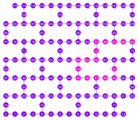
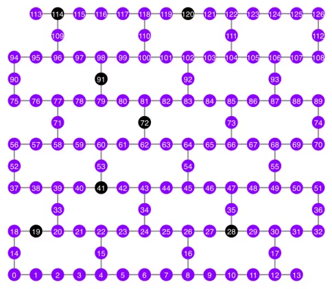
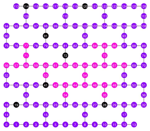
I-plot natin ang pinakamahusay na qubit chain, na ipinapakita sa kulay pink, sa diagram ng coupling map.

qubit_color = []
for i in range(133):
    if i in best_qubit_chain:
        qubit_color.append("#ff00dd")  # pink
    else:
        qubit_color.append("#8c00ff")  # purple
plot_gate_map(
    backend, qubit_color=qubit_color, qubit_size=50, font_size=25, figsize=(6, 6)
)

2.1 Bumuo ng GHZ circuit sa pinakamahusay na qubit chain

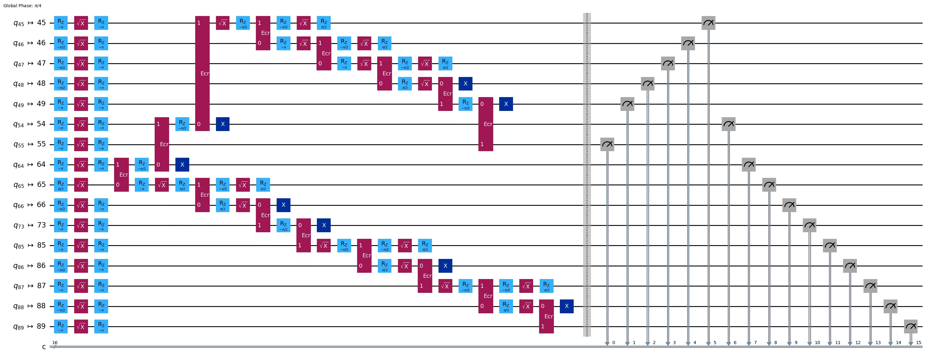
Pumipili tayo ng qubit sa gitna ng chain upang munang ilapat ang H gate dito. Dapat nitong mabawasan ang depth ng circuit ng halos kalahati.

ghz1 = QuantumCircuit(max(best_qubit_chain) + 1, N)
ghz1.h(best_qubit_chain[N // 2])
for i in range(N // 2, 0, -1):
    ghz1.cx(best_qubit_chain[i], best_qubit_chain[i - 1])
for i in range(N // 2, N - 1, +1):
    ghz1.cx(best_qubit_chain[i], best_qubit_chain[i + 1])
ghz1.barrier()  # for visualization
ghz1.measure(best_qubit_chain, list(range(N)))
ghz1.draw(output="mpl", idle_wires=False, scale=0.5, fold=-1)

ghz1.depth()

10

pm = generate_preset_pass_manager(1, backend=backend)
ghz1_transpiled = pm.run(ghz1)
ghz1_transpiled.draw(output="mpl", idle_wires=False, fold=-1)

print("Depth:", ghz1_transpiled.depth())
print(
    "Two-qubit Depth:",
    ghz1_transpiled.depth(filter_function=lambda x: x.operation.num_qubits == 2),
)

Depth: 27
Two-qubit Depth: 8

opts = SamplerOptions()

res = execute_ghz_fidelity(
    ghz_circuit=ghz1,
    physical_qubits=best_qubit_chain,
    backend=backend,
    sampler_options=opts,
)

job_s = service.job(res[0])  # Use your job id showed above.
job_e = service.job(res[1])
print(job_s.status(), job_e.status())

DONE DONE

Mag-ingat na patakbuhin ang susunod na cell pagkatapos lamang na maging 'DONE' ang status ng mga job sa itaas, upang maipakita ang resulta gamit ang function na check_ghz_fidelity_from_jobs.

N = 16
# Check fidelity from job IDs
res = check_ghz_fidelity_from_jobs(
    sampler_job=job_s,
    estimator_job=job_e,
    num_qubits=N,
)

N=16: |00..0>: 153, |11..1>: 8681, |3rd>: 2262 (1111111111101111)
P(|00..0>)=0.003825, P(|11..1>)=0.217025
REM: Coherence (non-diagonal): 0.073809
GHZ fidelity = 0.147329 ± 0.002438
GME (genuinely multipartite entangled) test: Failed

result = job_s.result()
plot_histogram(result[0].data.c.get_counts(), figsize=(30, 5))

Hindi natutugunan ng resultang ito ang pamantayan. Pumunta tayo sa susunod na ideya.

3. Estratehiya 2. Balanced tree ng mga qubit

Ang susunod na ideya ay hanapin ang isang balanced tree ng mga qubit. Sa pamamagitan ng paggamit ng tree kaysa sa chain, mas mababa ang magiging circuit depth. Bago iyon, inaalis natin ang mga node na may "masamang" readout error at mga edge na may "masamang" gate error mula sa coupling graph.

BAD_READOUT_ERROR_THRESHOLD = 0.1
BAD_ECRGATE_ERROR_THRESHOLD = 0.1
bad_readout_qubits = [
    q
    for q in range(backend.num_qubits)
    if backend.target["measure"][(q,)].error > BAD_READOUT_ERROR_THRESHOLD
]
bad_ecrgate_edges = [
    qpair
    for qpair in backend.target["ecr"]
    if backend.target["ecr"][qpair].error > BAD_ECRGATE_ERROR_THRESHOLD
]
print("Bad readout qubits:", bad_readout_qubits)
print("Bad ECR gates:", bad_ecrgate_edges)

Bad readout qubits: [19, 28, 41, 72, 91, 114, 120]
Bad ECR gates: []

g = backend.coupling_map.graph.copy().to_undirected()
g.remove_edges_from(
    bad_ecrgate_edges
)  # remove edge first (otherwise might fail with a NoEdgeBetweenNodes error)
g.remove_nodes_from(bad_readout_qubits)

Iguhit natin ang coupling map graph nang wala ang mga masamang edge at masamang qubit.

qubit_color = []
for i in range(133):
    if i in bad_readout_qubits:
        qubit_color.append("#000000")  # black
    else:
        qubit_color.append("#8c00ff")  # purple
line_color = []
for e in backend.target.build_coupling_map().get_edges():
    if e in bad_ecrgate_edges:
        line_color.append("#ffffff")  # white
    else:
        line_color.append("#888888")  # gray
plot_gate_map(
    backend,
    qubit_color=qubit_color,
    line_color=line_color,
    qubit_size=50,
    font_size=25,
    figsize=(6, 6),
)

Subukan nating gumawa ng 16-qubit GHZ state tulad ng dati.

N = 16

Tinatawag natin ang betweenness_centrality function para mahanap ang isang qubit para sa root node. Ang node na may pinakamataas na betweenness centrality ay nasa gitna ng graph. Sanggunian: https://www.rustworkx.org/tutorial/betweenness_centrality.html

O maaari mo rin itong piliin nang manu-mano.

# central = 65 #Select the center node manually
c_degree = dict(rx.betweenness_centrality(g))
central = max(c_degree, key=c_degree.get)
central

66

Simula sa root node, gumawa ng tree gamit ang breadth first search (BFS). Sanggunian: https://qiskit.org/ecosystem/rustworkx/apiref/rustworkx.bfs_search.html#rustworkx-bfs-search

class TreeEdgesRecorder(rx.visit.BFSVisitor):
    def __init__(self, N):
        self.edges = []
        self.N = N

    def tree_edge(self, edge):
        self.edges.append(edge)
        if len(self.edges) >= self.N - 1:
            raise rx.visit.StopSearch()

vis = TreeEdgesRecorder(N)
rx.bfs_search(g, [central], vis)
best_qubits = sorted(list(set(q for e in vis.edges for q in (e[0], e[1]))))
# print('Tree edges:', vis.edges)

print("Qubits selected:", best_qubits)

Qubits selected: [54, 55, 63, 64, 65, 66, 67, 68, 69, 70, 73, 83, 84, 85, 86, 87]

Ipakita natin ang mga napiling qubit, na kulay pink, sa coupling map diagram.

qubit_color = []
for i in range(133):
    if i in bad_readout_qubits:
        qubit_color.append("#000000")  # black
    elif i in best_qubits:
        qubit_color.append("#ff00dd")  # pink
    else:
        qubit_color.append("#8c00ff")  # purple
plot_gate_map(
    backend,
    qubit_color=qubit_color,
    line_color=line_color,
    qubit_size=50,
    font_size=25,
    figsize=(6, 6),
)

Ipakita natin ang tree structure ng mga qubit.

from rustworkx.visualization import graphviz_draw

tree = rx.PyDiGraph()
tree.extend_from_weighted_edge_list(vis.edges)
tree.remove_nodes_from([n for n in range(max(best_qubits) + 1) if n not in best_qubits])

graphviz_draw(tree, method="dot")

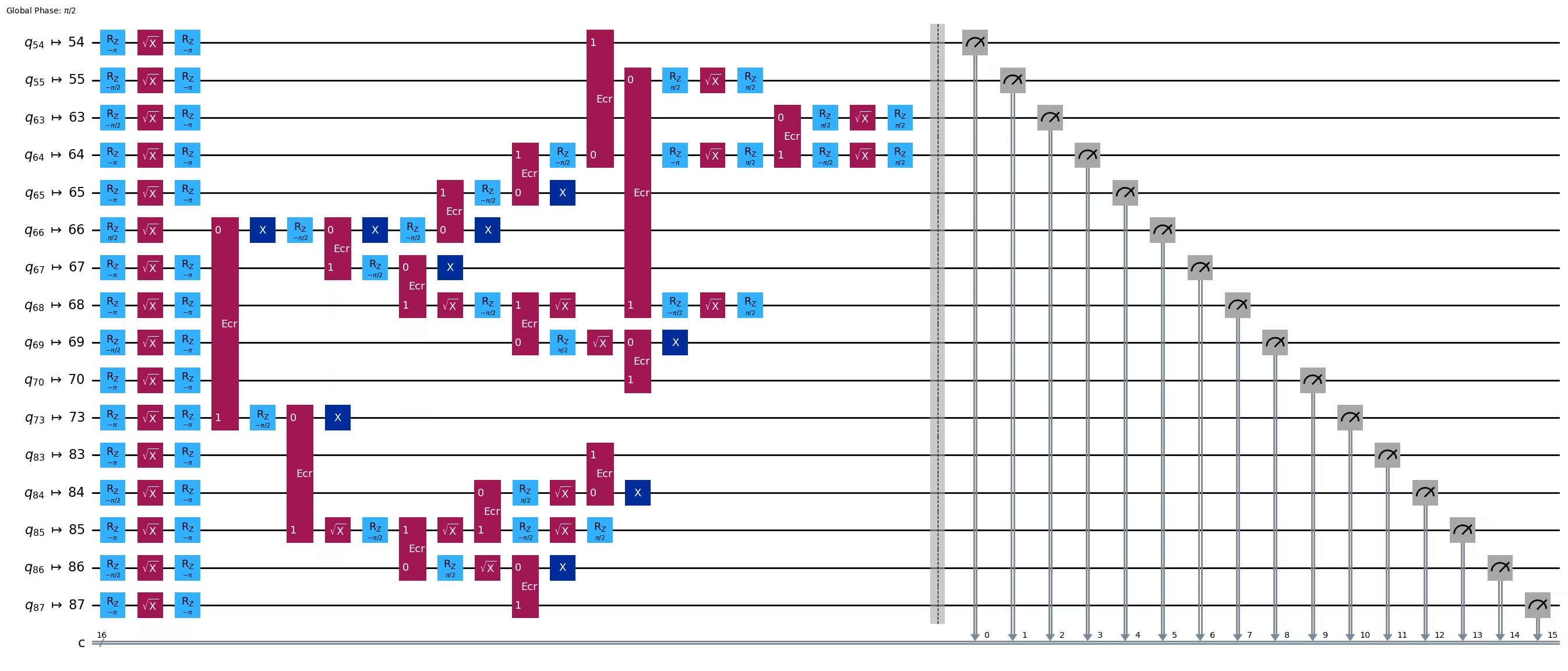
ghz2 = QuantumCircuit(max(best_qubits) + 1, N)

ghz2.h(tree.edge_list()[0][0])  # apply H-gate to the root node
# Apply CNOT from the root node to the each edge.
for u, v in tree.edge_list():
    ghz2.cx(u, v)
ghz2.barrier()  # for visualization
ghz2.measure(best_qubits, list(range(N)))
ghz2.draw(output="mpl", idle_wires=False, scale=0.5)

ghz2.depth()

8

pm = generate_preset_pass_manager(1, backend=backend)
ghz2_transpiled = pm.run(ghz2)
ghz2_transpiled.draw(output="mpl", idle_wires=False, fold=-1)

print("Depth:", ghz2_transpiled.depth())
print(
    "Two-qubit Depth:",
    ghz2_transpiled.depth(filter_function=lambda x: x.operation.num_qubits == 2),
)

Depth: 22
Two-qubit Depth: 6

Ang depth ng circuit ay naging mas mababa na kaysa sa chain structure.

res = execute_ghz_fidelity(
    ghz_circuit=ghz2,
    physical_qubits=best_qubits,
    backend=backend,
    sampler_options=opts,
)

job_s = service.job(res[0])  # Use your job id showed above.
job_e = service.job(res[1])
print(job_s.status(), job_e.status())

DONE DONE

N = 16
# Check fidelity from job IDs
res = check_ghz_fidelity_from_jobs(
    sampler_job=job_s,
    estimator_job=job_e,
    num_qubits=N,
)

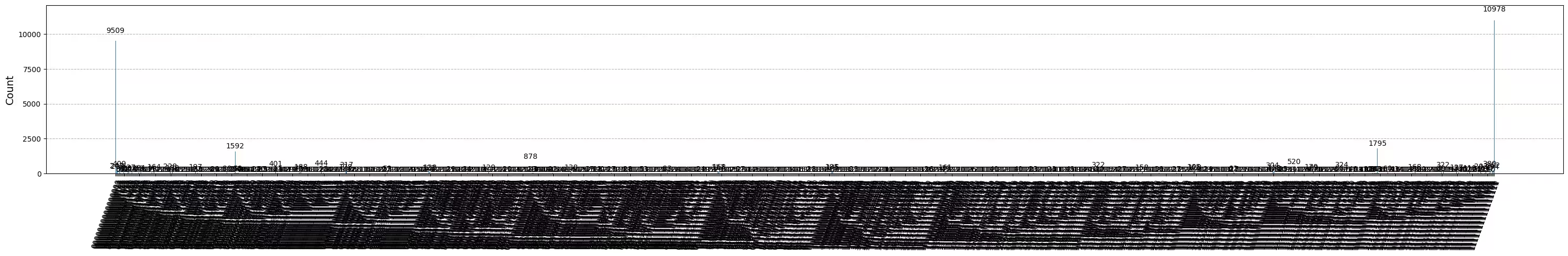
N=16: |00..0>: 9509, |11..1>: 10978, |3rd>: 1795 (1111110111111111)
P(|00..0>)=0.237725, P(|11..1>)=0.27445
REM: Coherence (non-diagonal): 0.606515
GHZ fidelity = 0.559345 ± 0.003188
GME (genuinely multipartite entangled) test: Passed

Matagumpay nating napasa ang pamantayan gamit ang balanced tree structure!

result = job_s.result()
plot_histogram(result[0].data.c.get_counts(), figsize=(30, 5))

Ngayon, subukan nating gumawa ng mas malaking GHZ state: isang 30-qubit GHZ state.

3.1 N = 30

Susundan natin ang Qiskit patterns framework.

• Hakbang 1: I-map ang problema sa mga quantum circuit at operator
• Hakbang 2: I-optimize para sa target na hardware
• Hakbang 3: Isagawa sa target na hardware
• Hakbang 4: I-post-process ang mga resulta

Hakbang 1: I-map ang problema sa mga quantum circuit at operator at Hakbang 2: I-optimize para sa target na hardware

Dito, manu-manong pipiliin natin ang root node.

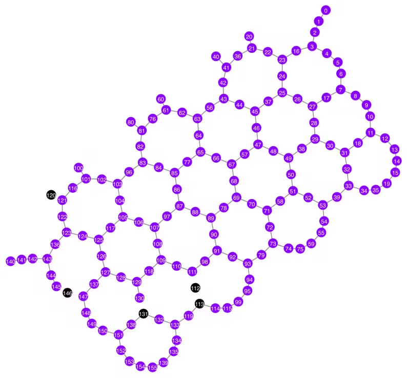
central = 62  # Select the center node manually
# c_degree = dict(rx.betweenness_centrality(g))
# central = max(c_degree, key=c_degree.get)
# central

N = 30

vis = TreeEdgesRecorder(N)
rx.bfs_search(g, [central], vis)
best_qubits = sorted(list(set(q for e in vis.edges for q in (e[0], e[1]))))
print("Qubits selected:", best_qubits)

Qubits selected: [34, 35, 42, 43, 44, 45, 46, 47, 48, 53, 54, 56, 57, 58, 59, 60, 61, 62, 63, 64, 65, 66, 67, 68, 71, 73, 77, 84, 85, 86]

qubit_color = []
for i in range(133):
    if i in bad_readout_qubits:
        qubit_color.append("#000000")
    elif i in best_qubits:
        qubit_color.append("#ff00dd")
    else:
        qubit_color.append("#8c00ff")
line_color = []
for e in backend.target.build_coupling_map().get_edges():
    if e in bad_ecrgate_edges:
        line_color.append("#ffffff")
    else:
        line_color.append("#888888")
plot_gate_map(
    backend,
    qubit_color=qubit_color,
    line_color=line_color,
    qubit_size=50,
    font_size=25,
    figsize=(6, 6),
)

from rustworkx.visualization import graphviz_draw

tree = rx.PyDiGraph()
tree.extend_from_weighted_edge_list(vis.edges)
tree.remove_nodes_from([n for n in range(max(best_qubits) + 1) if n not in best_qubits])

graphviz_draw(tree, method="dot")

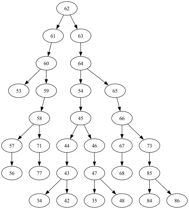
Ang depth ng tree na ito ay 5.

ghz3 = QuantumCircuit(max(best_qubits) + 1, N)

ghz3.h(tree.edge_list()[0][0])  # apply H-gate to the root node
# Apply CNOT from the root node to the each edge.
for u, v in tree.edge_list():
    ghz3.cx(u, v)
ghz3.barrier()  # for visualization
ghz3.measure(best_qubits, list(range(N)))
ghz3.draw(output="mpl", idle_wires=False, fold=-1)

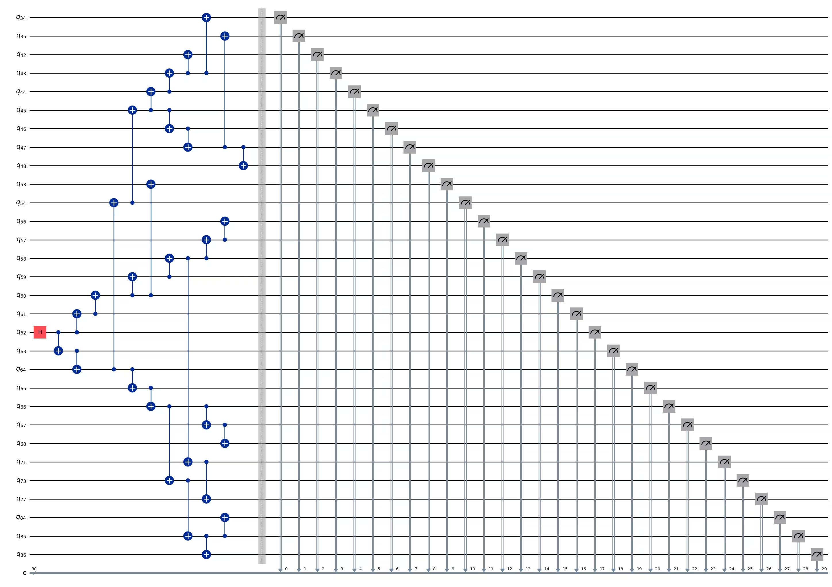
ghz3.depth()

11

pm = generate_preset_pass_manager(1, backend=backend)
ghz3_transpiled = pm.run(ghz3)
ghz3_transpiled.draw(output="mpl", idle_wires=False, fold=-1)

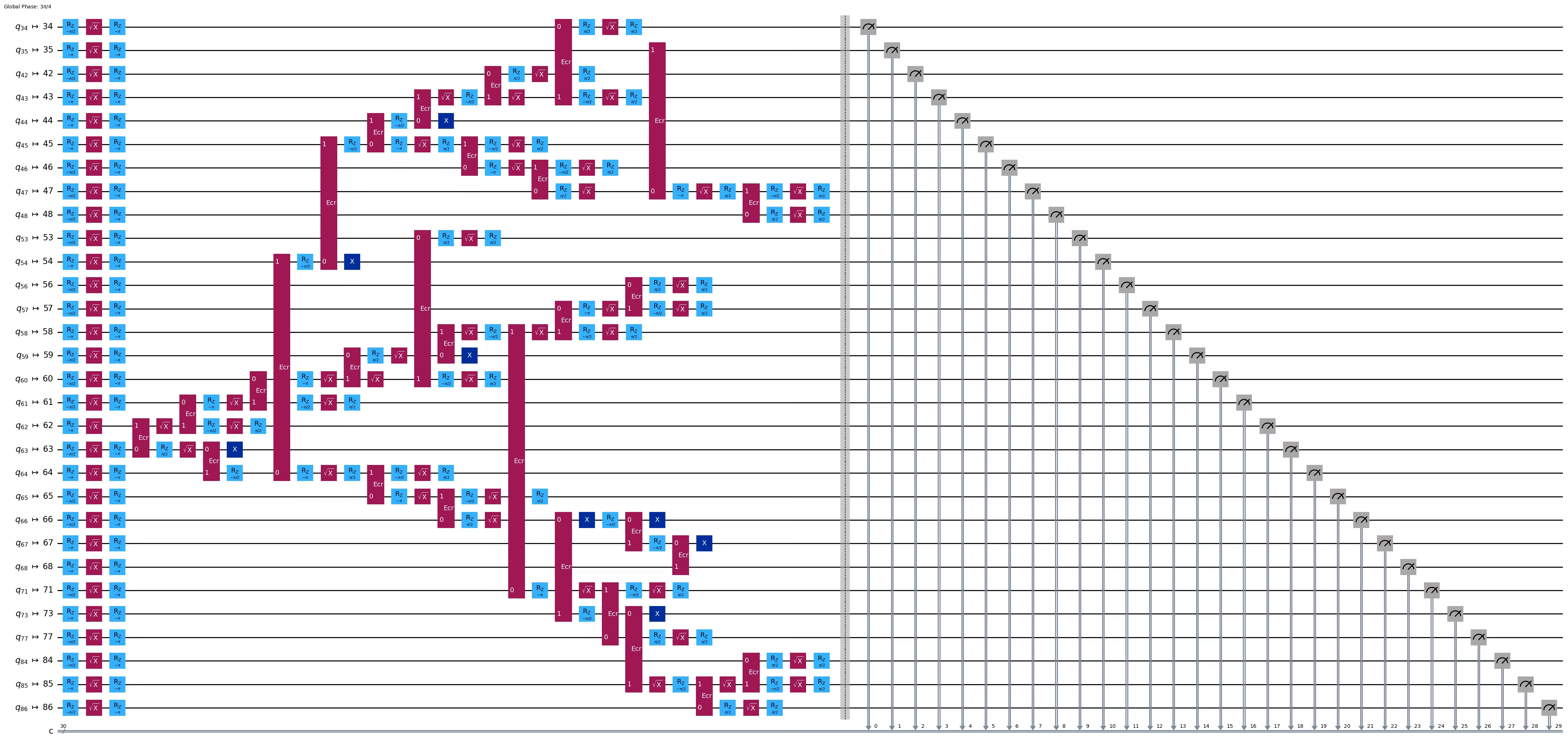
print("Depth:", ghz3_transpiled.depth())
print(
    "Two-qubit Depth:",
    ghz3_transpiled.depth(filter_function=lambda x: x.operation.num_qubits == 2),
)

Depth: 31
Two-qubit Depth: 9

3.2 Pumili ng ibang root node nang manu-mano

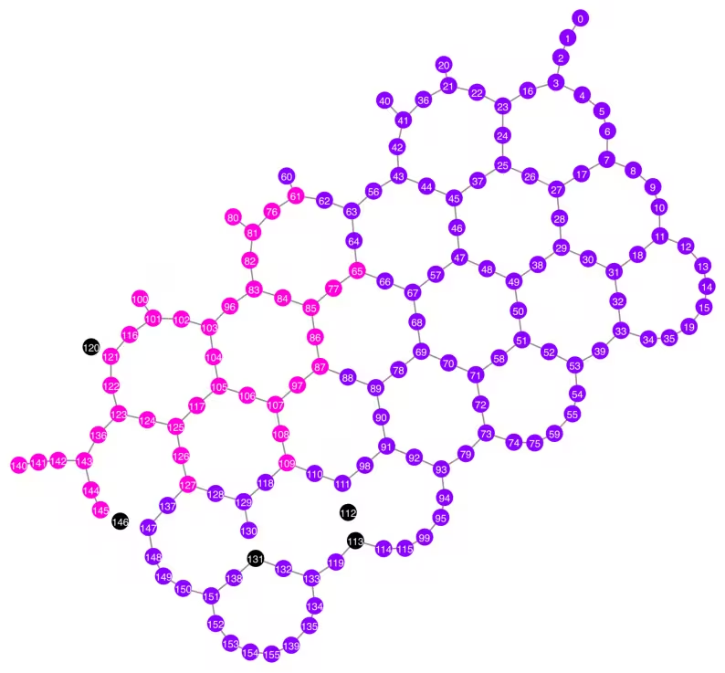
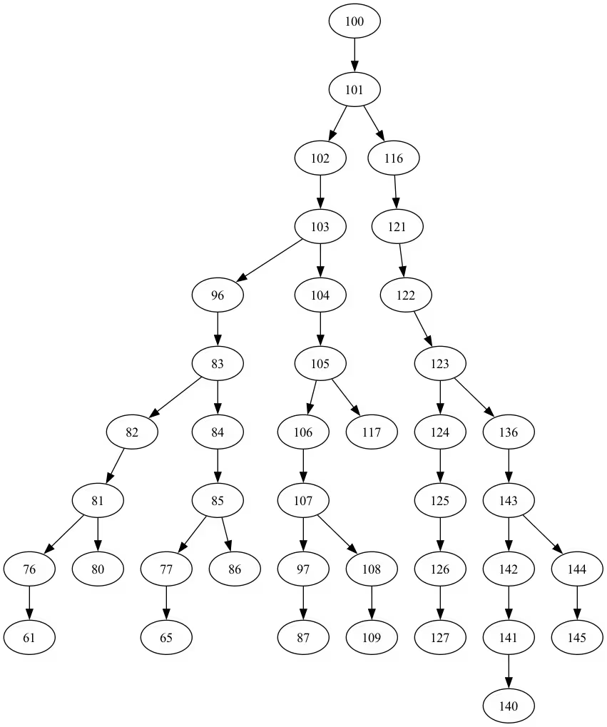
central = 54

vis = TreeEdgesRecorder(N)
rx.bfs_search(g, [central], vis)
best_qubits = sorted(list(set(q for e in vis.edges for q in (e[0], e[1]))))
print("Qubits selected:", best_qubits)

Qubits selected: [23, 24, 25, 34, 35, 42, 43, 44, 45, 46, 47, 48, 49, 50, 54, 55, 60, 61, 62, 63, 64, 65, 66, 67, 68, 69, 73, 84, 85, 86]

from rustworkx.visualization import graphviz_draw

tree = rx.PyDiGraph()
tree.extend_from_weighted_edge_list(vis.edges)
tree.remove_nodes_from([n for n in range(max(best_qubits) + 1) if n not in best_qubits])

graphviz_draw(tree, method="dot")

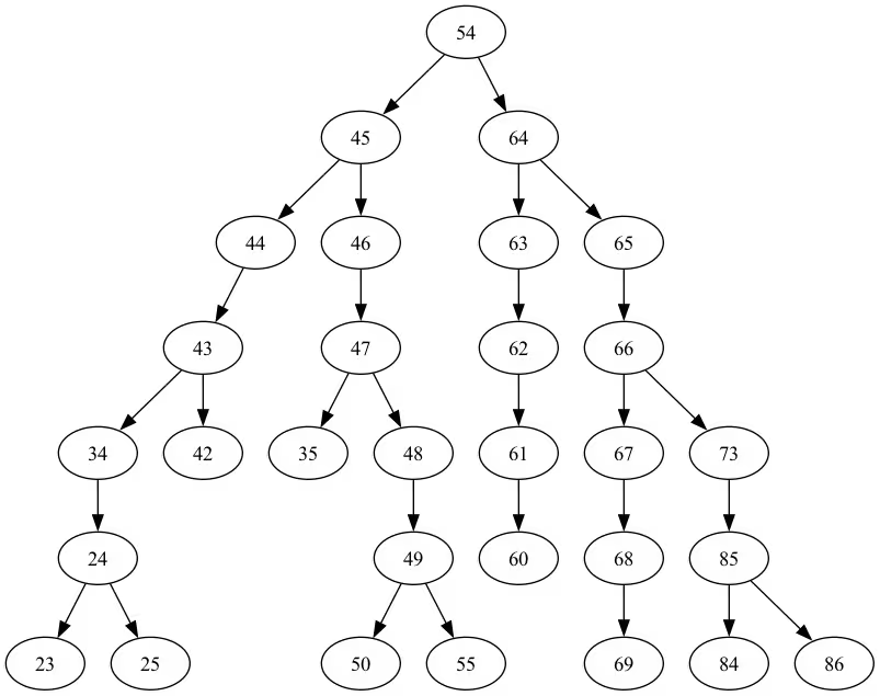
Ang depth ng tree na ito ay 6.

ghz3 = QuantumCircuit(max(best_qubits) + 1, N)

ghz3.h(tree.edge_list()[0][0])  # apply H-gate to the root node
# Apply CNOT from the root node to the each edge.
for u, v in tree.edge_list():
    ghz3.cx(u, v)
ghz3.barrier()  # for visualization
ghz3.measure(best_qubits, list(range(N)))
ghz3.draw(output="mpl", idle_wires=False, fold=-1)

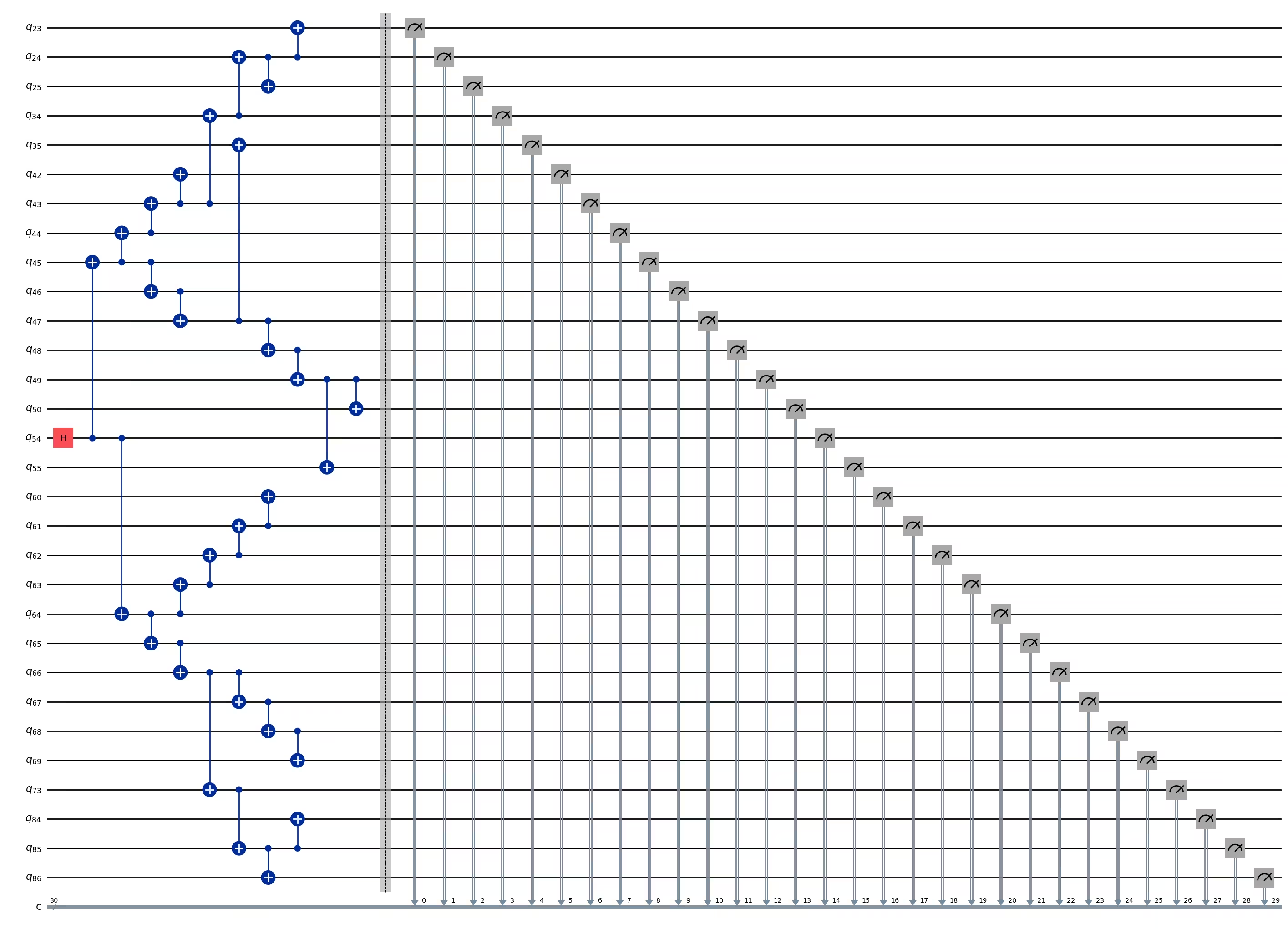
ghz3.depth()

11

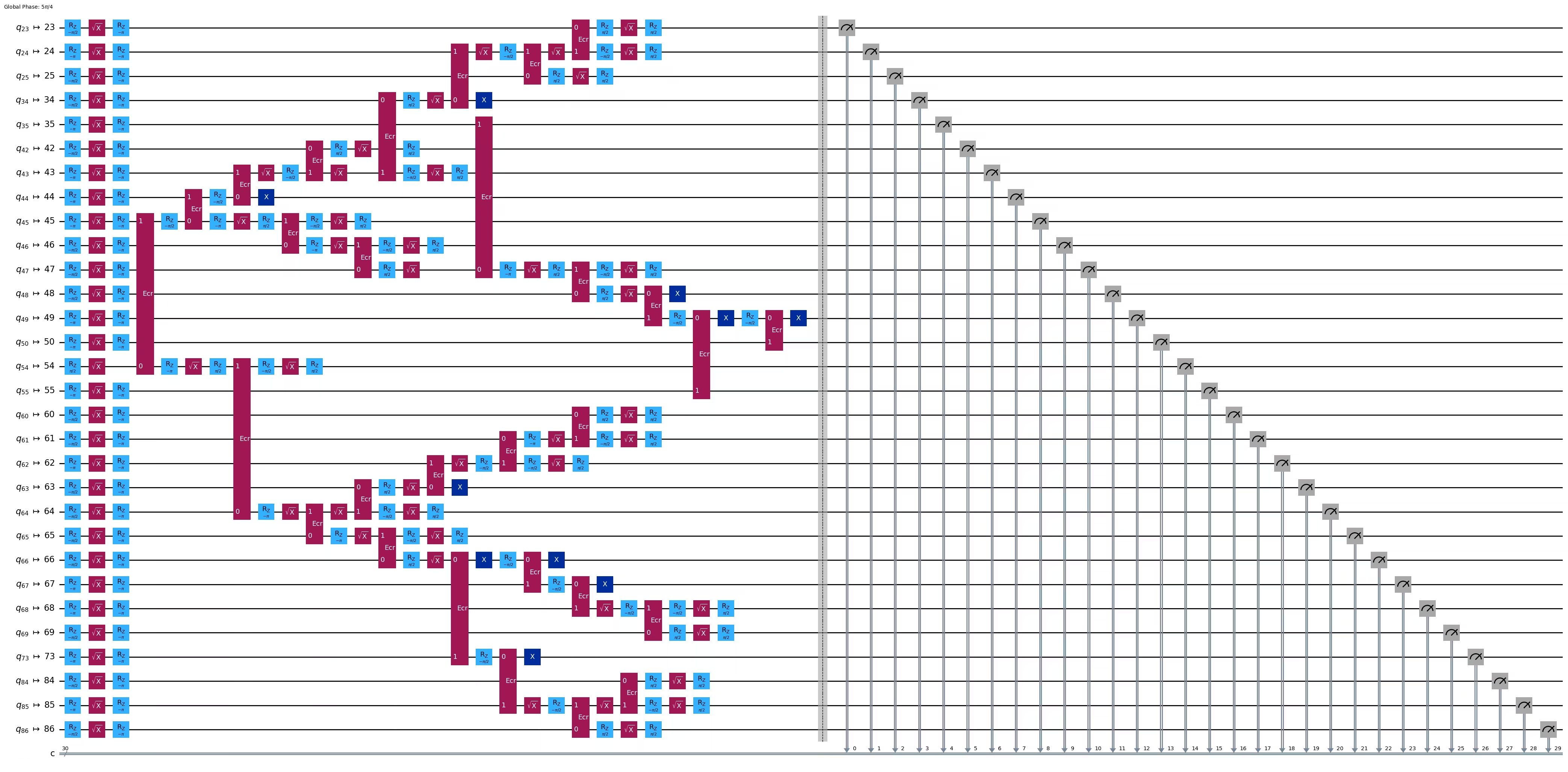
pm = generate_preset_pass_manager(1, backend=backend)
ghz3_transpiled = pm.run(ghz3)
ghz3_transpiled.draw(output="mpl", idle_wires=False, fold=-1)

print("Depth:", ghz3_transpiled.depth())
print(
    "Two-qubit Depth:",
    ghz3_transpiled.depth(filter_function=lambda x: x.operation.num_qubits == 2),
)

Depth: 30
Two-qubit Depth: 9

Kahanga-hanga, kahit na tumaas ang tree depth mula 5 hanggang 6, bumaba ang two-qubit depth mula 9 hanggang 8! Kaya gamitin natin ang huli na circuit.

Hakbang 3: Isagawa sa target na hardware

res = execute_ghz_fidelity(
    ghz_circuit=ghz3,
    physical_qubits=best_qubits,
    backend=backend,
    sampler_options=opts,
)

job_s = service.job(res[0])  # Use your job id showed above.
job_e = service.job(res[1])
print(job_s.status(), job_e.status())

DONE DONE

Hakbang 4: I-post-process ang mga resulta

N = 30
# Check fidelity from job IDs
res = check_ghz_fidelity_from_jobs(
    sampler_job=job_s,
    estimator_job=job_e,
    num_qubits=N,
)

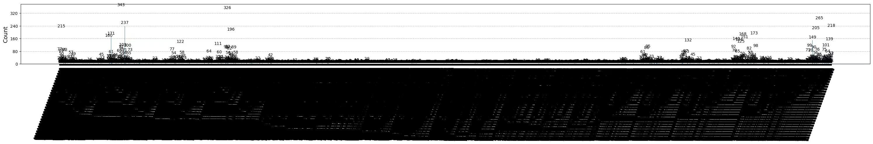
N=30: |00..0>: 4, |11..1>: 218, |3rd>: 265 (111111111111111011111111111111)
P(|00..0>)=0.0001, P(|11..1>)=0.00545
REM: Coherence (non-diagonal): 0.187073
GHZ fidelity = 0.096312 ± 0.003254
GME (genuinely multipartite entangled) test: Failed

Makikita mo na hindi natugunan ng resultang ito ang pamantayan.

# It will take some time
result = job_s.result()
plot_histogram(result[0].data.c.get_counts(), figsize=(30, 5))

4. Estratehiya 3. Patakbuhin gamit ang mga opsyon sa pag-suppress ng error

Maaari kang magtakda ng mga opsyon sa pag-suppress ng error sa Sampler V2. Tingnan ang gabay na Configure error mitigation at ang ExecutionOptionsV2 API reference para sa karagdagang impormasyon.

opts = SamplerOptions()
opts.dynamical_decoupling.enable = True
opts.execution.rep_delay = 0.0005
opts.twirling.enable_gates = True

res = execute_ghz_fidelity(
    ghz_circuit=ghz3,
    physical_qubits=best_qubits,
    backend=backend,
    sampler_options=opts,
)

job_s = service.job(res[0])  # Use your job id showed above.
job_e = service.job(res[1])
print(job_s.status(), job_e.status())

DONE DONE

N = 30

# Check fidelity from job IDs
res = check_ghz_fidelity_from_jobs(
    sampler_job=job_s,
    estimator_job=job_e,
    num_qubits=N,
)

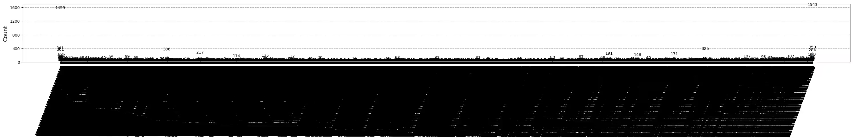
N=30: |00..0>: 1459, |11..1>: 1543, |3rd>: 359 (111111111111111111111111111110)
P(|00..0>)=0.036475, P(|11..1>)=0.038575
REM: Coherence (non-diagonal): 0.165532
GHZ fidelity = 0.120291 ± 0.003369
GME (genuinely multipartite entangled) test: Failed

# It will take some time
result = job_s.result()
plot_histogram(result[0].data.c.get_counts(), figsize=(30, 5))

Bumuti ang resulta ngunit hindi pa rin natutugunan ang pamantayan.

Nakita natin ang tatlong ideya sa ngayon. Maaari mong pagsamahin at palawakin ang mga ideyang ito, o makakalikha ka ng sarili mong mga ideya para gumawa ng mas mahusay na GHZ circuit. Ngayon, balikan natin ang layunin.

5. Ang iyong layunin (buod)

Gumawa ng GHZ circuit para sa 20 qubit o higit pa upang matugunan ang pamantayan: Ang fidelity ng iyong GHZ state ay > 0.5.

• Kailangan mong gumamit ng Eagle device (tulad ng ibm_brisbane) at itakda ang bilang ng shots sa 40,000.
• Dapat mong patakbuhin ang GHZ circuit gamit ang function na execute_ghz_fidelity, at kalkulahin ang fidelity gamit ang function na check_ghz_fidelity_from_jobs. Kailangan mong hanapin ang pinakamalaking GHZ circuit na nakakatugon sa pamantayan. Isulat ang iyong code sa ibaba, at ipakita ang resulta gamit ang function na check_ghz_fidelity_from_jobs.

Ngayon, ipapatupad natin ang parehong GHZ workflow tulad ng sa nakaraang materyal, ngunit sa isang Heron device. Magbibigay ito sa iyo ng karanasan sa layout at mga tampok ng mga Heron processor. Walang bagong estratehiya ang ipinakilala.

Ang tinatayang oras ng QPU para patakbuhin ang susunod na eksperimento ay 4 m 40 s.

service = QiskitRuntimeService()
backend = service.backend("ibm_kingston")
# backend = service.backend("ibm_fez")

twoq_gate = "cz"
print(f"Device {backend.name} Loaded with {backend.num_qubits} qubits")
print(f"Two Qubit Gate: {twoq_gate}")

Device ibm_kingston Loaded with 156 qubits
Two Qubit Gate: cz

BAD_READOUT_ERROR_THRESHOLD = 0.1
BAD_CZGATE_ERROR_THRESHOLD = 0.1
bad_readout_qubits = [
    q
    for q in range(backend.num_qubits)
    if backend.target["measure"][(q,)].error > BAD_READOUT_ERROR_THRESHOLD
]
bad_czgate_edges = [
    qpair
    for qpair in backend.target["cz"]
    if backend.target["cz"][qpair].error > BAD_CZGATE_ERROR_THRESHOLD
]
print("Bad readout qubits:", bad_readout_qubits)
print("Bad CZ gates:", bad_czgate_edges)

Bad readout qubits: [112, 113, 120, 131, 146]
Bad CZ gates: [(111, 112), (112, 111), (112, 113), (113, 112), (120, 121), (121, 120), (130, 131), (131, 130), (145, 146), (146, 145), (146, 147), (147, 146)]

g = backend.coupling_map.graph.copy().to_undirected()
g.remove_edges_from(
    bad_czgate_edges
)  # remove edge first (otherwise might fail with a NoEdgeBetweenNodes error)
g.remove_nodes_from(bad_readout_qubits)

qubit_color = []
for i in range(backend.num_qubits):
    if i in bad_readout_qubits:
        qubit_color.append("#000000")  # black
    else:
        qubit_color.append("#8c00ff")  # purple
line_color = []
for e in backend.target.build_coupling_map().get_edges():
    if e in bad_czgate_edges:
        line_color.append("#ffffff")  # white
    else:
        line_color.append("#888888")  # gray
plot_gate_map(
    backend,
    qubit_color=qubit_color,
    line_color=line_color,
    qubit_size=60,
    font_size=30,
    figsize=(10, 10),
)

N = 40
central = 100  # Select the center node manually
# c_degree = dict(rx.betweenness_centrality(g))
# central = max(c_degree, key=c_degree.get)
# central

class TreeEdgesRecorder(rx.visit.BFSVisitor):
    def __init__(self, N):
        self.edges = []
        self.N = N

    def tree_edge(self, edge):
        self.edges.append(edge)
        if len(self.edges) >= self.N - 1:
            raise rx.visit.StopSearch()

vis = TreeEdgesRecorder(N)
rx.bfs_search(g, [central], vis)
best_qubits = sorted(list(set(q for e in vis.edges for q in (e[0], e[1]))))
print("Qubits selected:", best_qubits)

Qubits selected: [61, 65, 76, 77, 80, 81, 82, 83, 84, 85, 86, 87, 96, 97, 100, 101, 102, 103, 104, 105, 106, 107, 108, 109, 116, 117, 121, 122, 123, 124, 125, 126, 127, 136, 140, 141, 142, 143, 144, 145]

qubit_color = []
for i in range(backend.num_qubits):
    if i in bad_readout_qubits:
        qubit_color.append("#000000")
    elif i in best_qubits:
        qubit_color.append("#ff00dd")
    else:
        qubit_color.append("#8c00ff")
line_color = []
for e in backend.target.build_coupling_map().get_edges():
    if e in bad_czgate_edges:
        line_color.append("#ffffff")
    else:
        line_color.append("#888888")
plot_gate_map(
    backend,
    qubit_color=qubit_color,
    line_color=line_color,
    qubit_size=60,
    font_size=30,
    figsize=(10, 10),
)

from rustworkx.visualization import graphviz_draw

tree = rx.PyDiGraph()
tree.extend_from_weighted_edge_list(vis.edges)
tree.remove_nodes_from([n for n in range(max(best_qubits) + 1) if n not in best_qubits])

graphviz_draw(tree, method="dot")

ghz_h = QuantumCircuit(max(best_qubits) + 1, N)

ghz_h.h(tree.edge_list()[0][0])  # apply H-gate to the root node
# Apply CNOT from the root node to the each edge.
for u, v in tree.edge_list():
    ghz_h.cx(u, v)
ghz_h.barrier()  # for visualization
ghz_h.measure(best_qubits, list(range(N)))
ghz_h.draw(output="mpl", idle_wires=False, fold=-1)

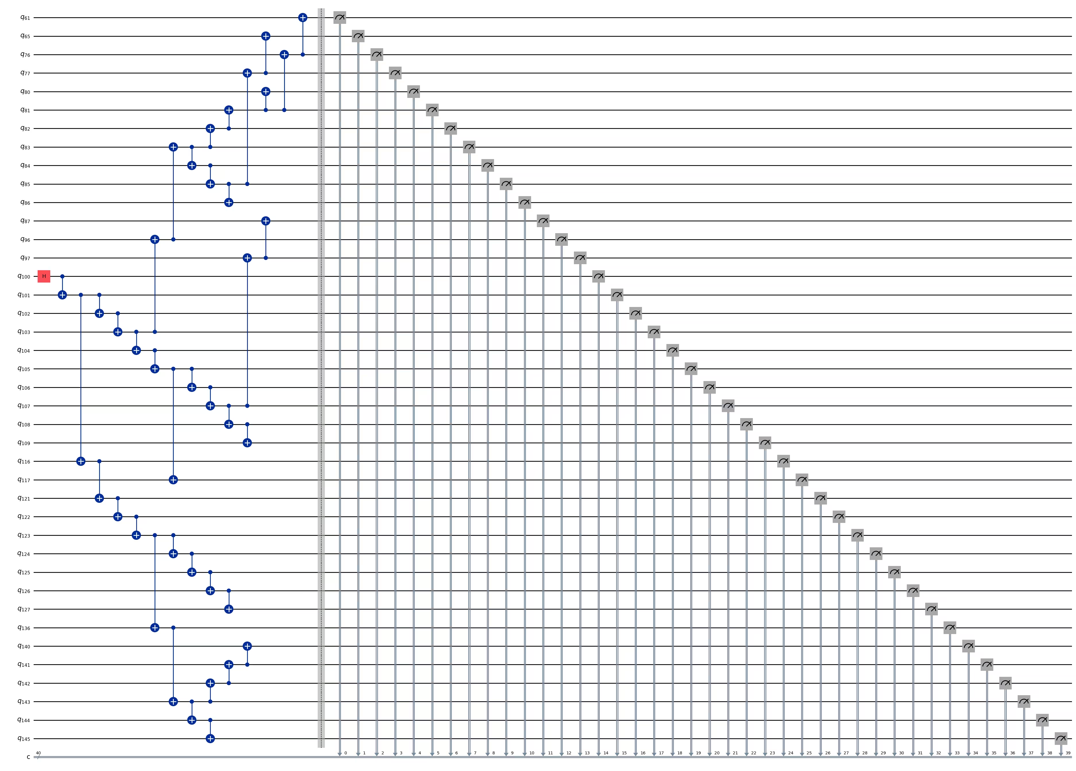
ghz_h.depth()

15

pm = generate_preset_pass_manager(1, backend=backend)
ghz_h_transpiled = pm.run(ghz_h)
ghz_h_transpiled.draw(output="mpl", idle_wires=False, fold=-1)

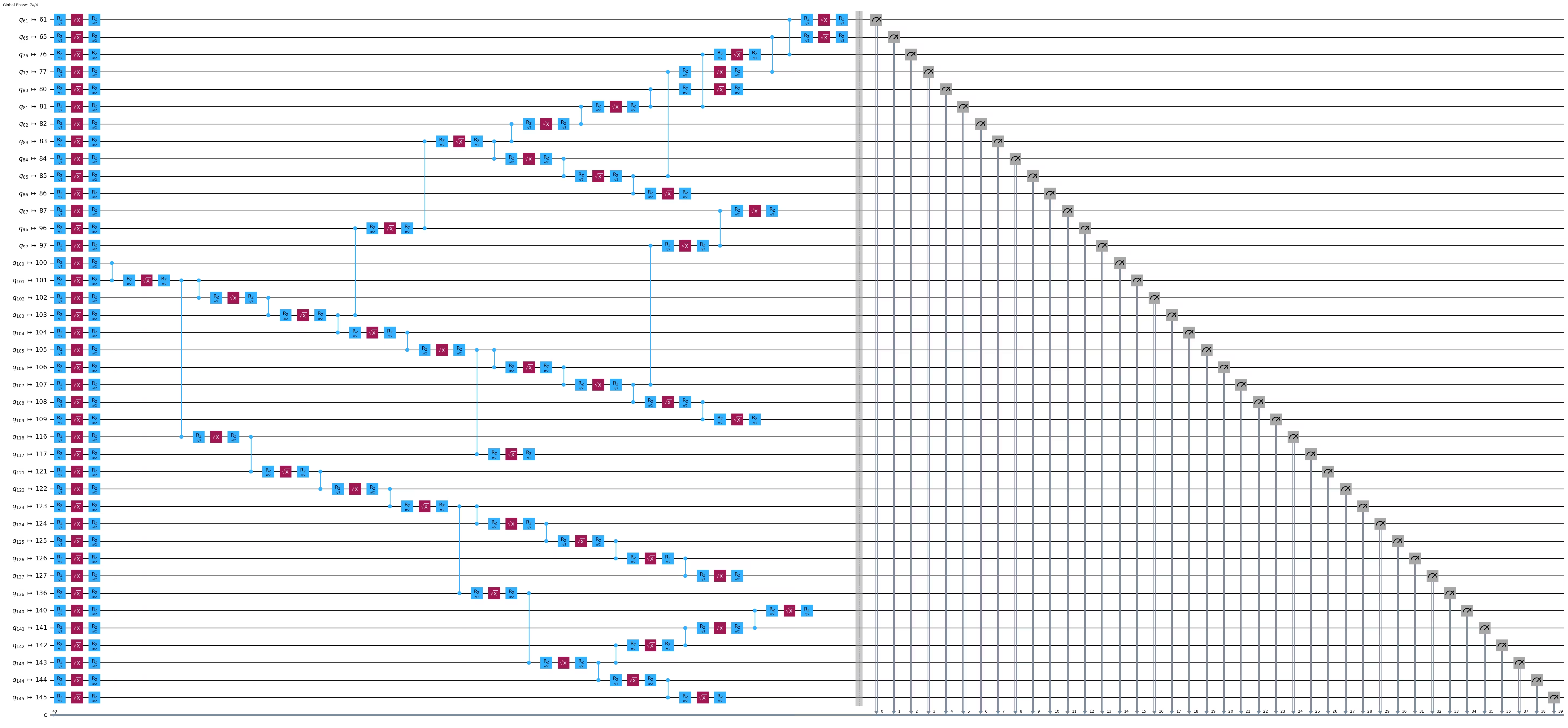
print("Depth:", ghz_h_transpiled.depth())
print(
    "Two-qubit Depth:",
    ghz_h_transpiled.depth(filter_function=lambda x: x.operation.num_qubits == 2),
)

Depth: 45
Two-qubit Depth: 13

opts = SamplerOptions()
opts.dynamical_decoupling.enable = True
opts.execution.rep_delay = 0.0005
opts.twirling.enable_gates = True

res = execute_ghz_fidelity(
    ghz_circuit=ghz_h,
    physical_qubits=best_qubits,
    backend=backend,
    sampler_options=opts,
)

job_s = service.job(res[0])  # Use your job id showed above.
job_e = service.job(res[1])
print(job_s.status(), job_e.status())

RUNNING RUNNING

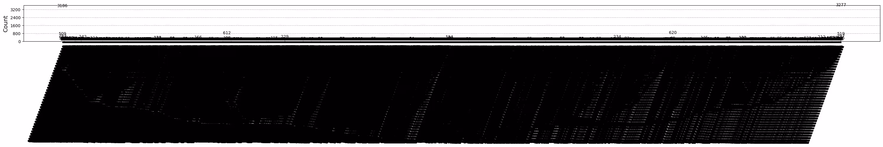
# Check fidelity from job IDs
N = 40
res = check_ghz_fidelity_from_jobs(
    sampler_job=job_s,
    estimator_job=job_e,
    num_qubits=N,
)

N=40: |00..0>: 3186, |11..1>: 3277, |3rd>: 620 (1111111011111111111111111111111111111111)
P(|00..0>)=0.07965, P(|11..1>)=0.081925
REM: Coherence (non-diagonal): 0.029987
GHZ fidelity = 0.095781 ± 0.002619
GME (genuinely multipartite entangled) test: Failed

# It will take some time
result = job_s.result()
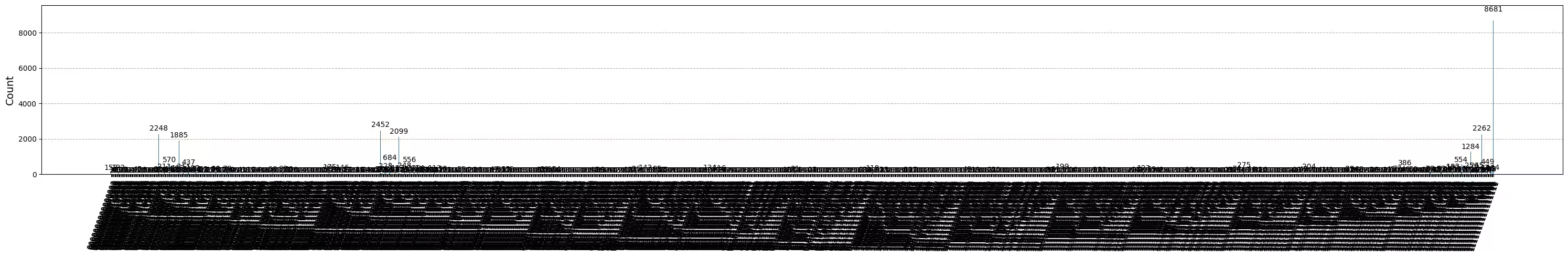
plot_histogram(result[0].data.c.get_counts(), figsize=(30, 5))

Binabati kita! Natapos mo na ang iyong panimula sa utility-scale quantum computing! Handa ka na ngayong mag-ambag nang may kabuluhan sa paghahanap ng quantum advantage! Salamat sa pagiging bahagi ng IBM Quantum® sa iyong personal na quantum journey.

Survey pagkatapos ng kurso

Congratulations on completing this course! Please take a moment to help us improve our course by filling out the following quick survey. Your feedback will be used to enhance our content offering and user experience. Thank you!