Quantum simulation

tala

Yukio Kawashima (May 30, 2024)

I-download ang pdf ng orihinal na lektura. Tandaan na ang ilang mga code snippet ay maaaring maging deprecated dahil mga static na imahe ang mga ito.

Ang tinatayang oras ng QPU para patakbuhin ang eksperimentong ito ay 7 segundo.

(Ang notebook na ito ay halos kinuha mula sa isang na-deprecated na tutorial notebook para sa Qiskit Algorithms.)

1. Panimula

Bilang isang teknik para sa real-time na ebolusyon, ang Trotterization ay binubuo ng sunud-sunod na aplikasyon ng isang quantum gate o mga gate, na pinili upang mapalapitan ang ebolusyon ng sistema sa paglipas ng panahon para sa isang time slice. Batay sa ekwasyon ng Schrödinger, ang ebolusyon ng isang sistema na nagsimula sa estado $\vert\psi(0)\rangle$ ay may ganitong anyo:

\vert \psi(t) \rangle = e^{-i H t} \vert \psi(0) \rangle \text{,}

kung saan ang $H$ ay ang time-independent na Hamiltonian na namamahala sa sistema. Isinasaalang-alang natin ang isang Hamiltonian na maaaring isulat bilang isang weighted sum ng mga Pauli term na $H=\sum_j a_j P_j$ , kung saan ang $P_j$ ay kumakatawan sa tensor product ng mga Pauli term na kumikilos sa $n$ qubits. Sa partikular, ang mga Pauli term na ito ay maaaring mag-commute sa isa't isa, o hindi. Kapag ibinigay ang isang estado sa oras na $t=0$ , paano natin makukuha ang estado ng sistema sa susunod na oras na $|\psi(t)\rangle$ gamit ang isang quantum computer? Ang exponential ng isang operator ay pinakamadaling maunawaang sa pamamagitan ng Taylor series nito:

e^{-i H t} = 1-iHt-\frac{1}{2}H^2t^2+...

Ang ilang napaka-simpleng exponential, tulad ng $e^{iZ}$ , ay madaling maipatupad sa mga quantum computer gamit ang isang maliit na hanay ng mga quantum gate. Karamihan sa mga Hamiltonian na interesado tayo ay hindi magkakaroon ng iisang term lamang, kundi maraming term. Pansinin kung ano ang mangyayari kapag $H = H_1+H_2$ :

e^{-i H t} = 1-i(H_1+H_2)t-\frac{1}{2}(H_1+H_2)^2t^2+...

Kapag nag-commute ang $H_1$ at $H_2$ , mayroon tayong pamilyar na kaso (na totoo rin para sa mga numero, at sa mga variable na $a$ at $b$ sa ibaba):

e^{-i (a+b) t} = e^{-i a t}e^{-i b t}

Ngunit kapag hindi nag-commute ang mga operator, ang mga term ay hindi maaaring muling ayusin sa Taylor series upang ma-simplify sa ganitong paraan. Kaya naman, ang pagpapahayag ng mga kumplikadong Hamiltonian sa mga quantum gate ay isang hamon.

Ang isang solusyon ay isaalang-alang ang napakaliit na oras na $t$ , upang ang first-order term sa Taylor expansion ang mangibabaw. Sa ilalim ng pagpapalagay na iyon:

e^{-i (H_1+H_2) t} \approx 1-i(H_1+H_2)t \approx (1-i H_1 t)(1-i H_2 t) \approx e^{-i H_1 t}e^{-i H_2 t}

Siyempre, maaaring kailangan nating paunlarin ang ating estado para sa mas matagal na panahon. Ito ay nagagawa sa pamamagitan ng paggamit ng maraming maliliit na hakbang sa oras. Ang prosesong ito ay tinatawag na Trotterization:

\vert \psi(t) \rangle \approx \left(\prod_j e^{-i a_j P_j t/r} \right)^r \vert\psi(0) \rangle \text{,}

Dito, ang $t/r$ ay ang time slice (evolution step) na pinipili natin. Bilang resulta, isang gate ang nalilikha na ilalapat nang $r$ beses. Ang mas maliit na timestep ay nagdudulot ng mas tumpak na pagpapalapita. Gayunpaman, nagdudulot din ito ng mas malalim na circuits na, sa praktika, ay nagdudulot ng mas maraming error accumulation (isang hindi mapapabayaang alalahanin sa mga near-term na quantum device).

Sa araw na ito, aaralin natin ang ebolusyon ng oras ng Ising model sa mga linear na lattice na may $N=2$ at $N=6$ na mga site. Ang mga lattice na ito ay binubuo ng isang hanay ng mga spin na $\sigma_i$ na nakikipag-ugnayan lamang sa kanilang pinakamalapit na mga kapitbahay. Ang mga spin na ito ay maaaring magkaroon ng dalawang oryentasyon: $\uparrow$ at $\downarrow$ , na katumbas ng magnetization na $+1$ at $-1$ ayon sa pagkakabanggit.

H = - J \sum_{i=0}^{N-2} Z_i Z_{i+1} - h \sum_{i=0}^{N-1} X_i \text{,}

kung saan ang $J$ ay naglalarawan ng interaction energy, at ang $h$ ang magnitude ng isang panlabas na field (sa x-direksyon sa itaas, ngunit babaguhin natin ito). Isulat natin ang ekspresyong ito gamit ang mga Pauli matrix, at isaalang-alang na ang panlabas na field ay may anggulo na $\alpha$ kaugnay ng transversal na direksyon,

H = -J \sum_{i=0}^{N-2} Z_i Z_{i+1} -h \sum_{i=0}^{N-1} (\sin\alpha Z_i + \cos\alpha X_i) \text{.}

Ang Hamiltoniang ito ay kapaki-pakinabang dahil hinahayaan tayong madaling pag-aralan ang mga epekto ng isang panlabas na field. Sa computational basis, ang sistema ay ie-encode tulad ng sumusunod:

Quantum state	Representasyon ng Spin
$\lvert 0 0 0 0 \rangle$	$\uparrow\uparrow\uparrow\uparrow$
$\lvert 1 0 0 0 \rangle$	$\downarrow\uparrow\uparrow\uparrow$
$\ldots$	$\ldots$
$\lvert 1 1 1 1 \rangle$	$\downarrow\downarrow\downarrow\downarrow$

Magsisimula tayong pag-aralan ang ebolusyon ng oras ng ganitong quantum system. Mas partikular, i-visualize natin ang ebolusyon ng oras ng ilang katangian ng sistema tulad ng magnetization.

1.1 Mga Kinakailangan

Bago simulan ang tutorial na ito, siguraduhing naka-install ang mga sumusunod:

Qiskit SDK v1.2 o mas bago ( pip install qiskit )
Qiskit Runtime v0.30 o mas bago ( pip install qiskit-ibm-runtime )
Numpy v1.24.1 o mas bago < 2 ( pip install numpy )

1.2 I-import ang mga library

Tandaan na ang ilang library na maaaring makapaki-pakinabang (MatrixExponential, QDrift) ay kasama kahit hindi ginagamit sa kasalukuyang notebook. Subukan mo rin sila kapag may oras ka!

# Added by doQumentation — required packages for this notebook
!pip install -q matplotlib numpy qiskit qiskit-ibm-runtime

# Check the version of Qiskit
import qiskit

qiskit.__version__

'2.0.2'

# Import the qiskit library
import numpy as np
import matplotlib.pylab as plt
import warnings

from qiskit import QuantumCircuit
from qiskit.circuit.library import PauliEvolutionGate
from qiskit.primitives import StatevectorEstimator
from qiskit.quantum_info import Statevector, SparsePauliOp
from qiskit.synthesis import (
    SuzukiTrotter,
    LieTrotter,
)
from qiskit.transpiler.preset_passmanagers import generate_preset_pass_manager

from qiskit_ibm_runtime import QiskitRuntimeService, SamplerV2

warnings.filterwarnings("ignore")

2. Pag-map ng iyong problema

2.1 Pagtukoy sa transverse-field Ising Hamiltonian

Dito isinasaalang-alang natin ang 1-D transverse-field Ising model.

Una, lilikha tayo ng isang function na tumatanggap ng mga parameter ng sistema na $N$ , $J$ , $h$ at $\alpha$ , at nagbabalik ng ating Hamiltonian bilang isang SparsePauliOp. Ang isang SparsePauliOp ay isang sparse na representasyon ng isang operator sa mga tuntunin ng weighted na mga Pauli term.

def get_hamiltonian(nqubits, J, h, alpha):
    # List of Hamiltonian terms as 3-tuples containing
    # (1) the Pauli string,
    # (2) the qubit indices corresponding to the Pauli string,
    # (3) the coefficient.
    ZZ_tuples = [("ZZ", [i, i + 1], -J) for i in range(0, nqubits - 1)]
    Z_tuples = [("Z", [i], -h * np.sin(alpha)) for i in range(0, nqubits)]
    X_tuples = [("X", [i], -h * np.cos(alpha)) for i in range(0, nqubits)]

    # We create the Hamiltonian as a SparsePauliOp, via the method
    # `from_sparse_list`, and multiply by the interaction term.
    hamiltonian = SparsePauliOp.from_sparse_list(
        [*ZZ_tuples, *Z_tuples, *X_tuples], num_qubits=nqubits
    )
    return hamiltonian.simplify()

Tukuyin ang Hamiltonian

Ang sistema na isinasaalang-alang natin ngayon ay may sukat na $N=6$ , $J=0.2$ , $h=1.2$ at $\alpha=\frac{\pi}{8.0}$ bilang halimbawa.

n_qubits = 6

hamiltonian = get_hamiltonian(nqubits=n_qubits, J=0.2, h=1.2, alpha=np.pi / 8.0)
hamiltonian

SparsePauliOp(['IIIIZZ', 'IIIZZI', 'IIZZII', 'IZZIII', 'ZZIIII', 'IIIIIZ', 'IIIIZI', 'IIIZII', 'IIZIII', 'IZIIII', 'ZIIIII', 'IIIIIX', 'IIIIXI', 'IIIXII', 'IIXIII', 'IXIIII', 'XIIIII'],
              coeffs=[-0.2       +0.j, -0.2       +0.j, -0.2       +0.j, -0.2       +0.j,
 -0.2       +0.j, -0.45922012+0.j, -0.45922012+0.j, -0.45922012+0.j,
 -0.45922012+0.j, -0.45922012+0.j, -0.45922012+0.j, -1.10865544+0.j,
 -1.10865544+0.j, -1.10865544+0.j, -1.10865544+0.j, -1.10865544+0.j,
 -1.10865544+0.j])

2.2 Itakda ang mga parameter ng time-evolution simulation

Dito isasaalang-alang natin ang tatlong iba't ibang teknik ng Trotterization:

Lie–Trotter (first order)
second-order Suzuki–Trotter
fourth-order Suzuki–Trotter

Ang huli sa dalawa ay gagamitin sa ehersisyo, at sa appendix.

num_timesteps = 60
evolution_time = 30.0
dt = evolution_time / num_timesteps
product_formula_lt = LieTrotter()
product_formula_st2 = SuzukiTrotter(order=2)
product_formula_st4 = SuzukiTrotter(order=4)

2.3 Ihanda ang quantum circuit 1 (Paunang estado)

Lumikha ng paunang estado. Dito magsisimula tayo sa isang spin configuration na $\uparrow\uparrow\downarrow\downarrow\uparrow\uparrow$ .

initial_circuit = QuantumCircuit(n_qubits)
initial_circuit.prepare_state("001100")
# Change reps and see the difference when you decompose the circuit
initial_circuit.decompose(reps=1).draw("mpl")

Output of the previous code cell

2.4 Ihanda ang quantum circuit 2 (Iisang circuit para sa time evolution)

Dito gumagawa tayo ng circuit para sa iisang time step gamit ang Lie–Trotter.

Ang Lie product formula (first-order) ay ipinatupad sa klase na LieTrotter. Ang isang first-order formula ay binubuo ng pagpapalapita na binanggit sa panimula, kung saan ang matrix exponential ng isang sum ay pinapalapitan ng isang product ng mga matrix exponential:

e^{H_1+H_2} \approx e^{H_1} e^{H_2}

Tulad ng nabanggit na, ang napakalalim na mga circuit ay nagdudulot ng akumulasyon ng mga error, at nagdudulot ng mga problema para sa mga modernong quantum computer. Dahil ang mga two-qubit gate ay may mas mataas na rate ng error kaysa sa mga single-qubit gate, ang isang partikular na interesadong dami ay ang two-qubit circuit depth. Ang talagang mahalaga ay ang two-qubit circuit depth pagkatapos ng transpilation (dahil iyon ang circuit na talagang isinasagawa ng quantum computer). Ngunit ugaliing bilangin na natin ang mga operasyon para sa circuit na ito, kahit ngayon gamit ang simulator.

single_step_evolution_gates_lt = PauliEvolutionGate(
    hamiltonian, dt, synthesis=product_formula_lt
)
single_step_evolution_lt = QuantumCircuit(n_qubits)
single_step_evolution_lt.append(
    single_step_evolution_gates_lt, single_step_evolution_lt.qubits
)

print(
    f"""
Trotter step with Lie-Trotter
-----------------------------
Depth: {single_step_evolution_lt.decompose(reps=3).depth()}
Gate count: {len(single_step_evolution_lt.decompose(reps=3))}
Nonlocal gate count: {single_step_evolution_lt.decompose(reps=3).num_nonlocal_gates()}
Gate breakdown: {", ".join([f"{k.upper()}: {v}" for k, v in single_step_evolution_lt.decompose(reps=3).count_ops().items()])}
"""
)
single_step_evolution_lt.decompose(reps=3).draw("mpl", fold=-1)

Trotter step with Lie-Trotter
-----------------------------
Depth: 17
Gate count: 27
Nonlocal gate count: 10
Gate breakdown: U3: 12, CX: 10, U1: 5

Output of the previous code cell

2.5 Itakda ang mga operator na susukatin

Tukuyin natin ang isang magnetization operator na $\sum_i \langle Z_i \rangle / N$ , at isang mean spin correlation operator na $\sum_i \langle Z_i Z_{i+1} \rangle/ (N - 1)$ .

magnetization = (
    SparsePauliOp.from_sparse_list(
        [("Z", [i], 1.0) for i in range(0, n_qubits)], num_qubits=n_qubits
    )
    / n_qubits
)
correlation = SparsePauliOp.from_sparse_list(
    [("ZZ", [i, i + 1], 1.0) for i in range(0, n_qubits - 1)], num_qubits=n_qubits
) / (n_qubits - 1)
print("magnetization : ", magnetization)
print("correlation : ", correlation)

magnetization :  SparsePauliOp(['IIIIIZ', 'IIIIZI', 'IIIZII', 'IIZIII', 'IZIIII', 'ZIIIII'],
              coeffs=[0.16666667+0.j, 0.16666667+0.j, 0.16666667+0.j, 0.16666667+0.j,
 0.16666667+0.j, 0.16666667+0.j])
correlation :  SparsePauliOp(['IIIIZZ', 'IIIZZI', 'IIZZII', 'IZZIII', 'ZZIIII'],
              coeffs=[0.2+0.j, 0.2+0.j, 0.2+0.j, 0.2+0.j, 0.2+0.j])

2.6 Isagawa ang time-evolution simulation

Susubaybayan natin ang enerhiya (expectation value ng Hamiltonian), magnetization (expectation value ng magnetization operator), at mean spin correlation (expectation value ng mean spin correlation operator). Ang StatevectorEstimator (EstimatorV2) primitive ng Qiskit ay nagtatantya ng mga expectation value ng mga observable, $\langle\psi\vert\hat{O}\vert\psi\rangle$ .

# Initiate the circuit
evolved_state = QuantumCircuit(initial_circuit.num_qubits)
# Start from the initial spin configuration
evolved_state.append(initial_circuit, evolved_state.qubits)
# Initiate Estimator (V2)
estimator = StatevectorEstimator()
# Set number of shots
shots = 10000
# Translate the precision required from the number of shots
precision = np.sqrt(1 / shots)
energy_list = []
mag_list = []
corr_list = []
# Estimate expectation values for t=0.0
job = estimator.run(
    [(evolved_state, [hamiltonian, magnetization, correlation])], precision=precision
)
# Get estimated expectation values
evs = job.result()[0].data.evs
energy_list.append(evs[0])
mag_list.append(evs[1])
corr_list.append(evs[2])
# Start time evolution
for n in range(num_timesteps):
    # Expand the circuit to describe delta-t
    evolved_state.append(single_step_evolution_gates_lt, evolved_state.qubits)
    # Estimate expectation values at delta-t
    job = estimator.run(
        [(evolved_state, [hamiltonian, magnetization, correlation])],
        precision=precision,
    )
    # Retrieve results (expectation values)
    evs = job.result()[0].data.evs
    energy_list.append(evs[0])
    mag_list.append(evs[1])
    corr_list.append(evs[2])
# Transform the list of expectation values (at each time step) to arrays
energy_array = np.array(energy_list)
mag_array = np.array(mag_list)
corr_array = np.array(corr_list)

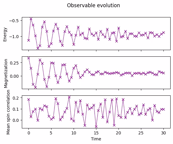
2.7 I-plot ang time evolution ng mga observable

Ipi-plot natin ang mga expectation value na sinukat natin laban sa oras.

fig, axes = plt.subplots(3, sharex=True)
times = np.linspace(0, evolution_time, num_timesteps + 1)  # includes initial state
axes[0].plot(
    times,
    energy_array,
    label="First order",
    marker="x",
    c="darkmagenta",
    ls="-",
    lw=0.8,
)
axes[1].plot(
    times, mag_array, label="First order", marker="x", c="darkmagenta", ls="-", lw=0.8
)
axes[2].plot(
    times, corr_array, label="First order", marker="x", c="darkmagenta", ls="-", lw=0.8
)
axes[0].set_ylabel("Energy")
axes[1].set_ylabel("Magnetization")
axes[2].set_ylabel("Mean spin correlation")
axes[2].set_xlabel("Time")
fig.suptitle("Observable evolution")

Text(0.5, 0.98, 'Observable evolution')

Output of the previous code cell

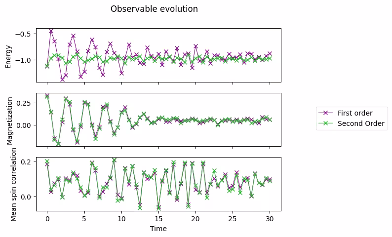
3. Ehersisyo 1. Magsagawa ng simulation gamit ang second-order Suzuki–Trotter

Subukan nating magsagawa ng simulation gamit ang second-order Suzuki–Trotter, na susunod sa halimbawa ng Lie–Trotter na ipinakita sa itaas.

Magagamit ang second-order Suzuki-Trotter sa Qiskit sa pamamagitan ng SuzukiTrotter class. Gamit ang formula na ito, ang second-order decomposition ay:

e^{H_1+H_2} \approx e^{H_1/2}e^{H_2}e^{H_1/2}

3.1 Bumuo ng circuit para sa isang time step

Gamitin ang product_formula_st2 (SuzukiTrotter(order=2)) at bumuo ng circuit para sa isang time step gamit ang second-order Suzuki–Trotter. Bilang karagdagan, bilangin ang mga gate at ang depth ng circuit, at ihambing ito sa Lie–Trotter.

# Modify the line below (Use PauliEvolutionGate)
single_step_evolution_gates_st2 = PauliEvolutionGate(
    hamiltonian, dt, synthesis=product_formula_st2
)
single_step_evolution_st2 = QuantumCircuit(n_qubits)
single_step_evolution_st2.append(
    single_step_evolution_gates_st2, single_step_evolution_st2.qubits
)
# Let us print some stats
print(
    f"""
Trotter step with second-order Suzuki-Trotter
-----------------------------
Depth: {single_step_evolution_st2.decompose(reps=3).depth()}
Gate count: {len(single_step_evolution_st2.decompose(reps=3))}
Nonlocal gate count: {single_step_evolution_st2.decompose(reps=3).num_nonlocal_gates()}
Gate breakdown: {", ".join([f"{k.upper()}: {v}" for k, v in single_step_evolution_st2.decompose(reps=3).count_ops().items()])}
"""
)
single_step_evolution_st2.decompose(reps=2).draw("mpl", fold=-1)

Trotter step with second-order Suzuki-Trotter
-----------------------------
Depth: 34
Gate count: 53
Nonlocal gate count: 20
Gate breakdown: U3: 23, CX: 20, U1: 10

Output of the previous code cell

3.2 Magsagawa ng time-evolution simulation

Magsagawa ng time evolution gamit ang second-order Suzuki–Trotter.

# Initiate the circuit
evolved_state = QuantumCircuit(initial_circuit.num_qubits)
# Start from the initial spin configuration
evolved_state.append(initial_circuit, evolved_state.qubits)
# Initiate Estimator (V2)
estimator = StatevectorEstimator()
# Set number of shots
shots = 10000
# Translate the precision required from the number of shots
precision = np.sqrt(1 / shots)
energy_list_st2 = []
mag_list_st2 = []
corr_list_st2 = []
# Estimate expectation values for t=0.0
job = estimator.run(
    [(evolved_state, [hamiltonian, magnetization, correlation])], precision=precision
)
# Get estimated expectation values
evs = job.result()[0].data.evs
energy_list_st2.append(evs[0])
mag_list_st2.append(evs[1])
corr_list_st2.append(evs[2])
# Start time evolution
for n in range(num_timesteps):
    # Expand the circuit to describe delta-t
    evolved_state.append(single_step_evolution_gates_st2, evolved_state.qubits)
    # Estimate expectation values at delta-t
    job = estimator.run(
        [(evolved_state, [hamiltonian, magnetization, correlation])],
        precision=precision,
    )
    # Retrieve results (expectation values)
    evs = job.result()[0].data.evs
    energy_list_st2.append(evs[0])
    mag_list_st2.append(evs[1])
    corr_list_st2.append(evs[2])
# Transform the list of expectation values (at each time step) to arrays
energy_array_st2 = np.array(energy_list_st2)
mag_array_st2 = np.array(mag_list_st2)
corr_array_st2 = np.array(corr_list_st2)

3.3 I-plot ang mga resulta ng second-order Suzuki–Trotter

axes[0].plot(
    times,
    energy_array_st2,
    label="Second Order",
    marker="x",
    c="limegreen",
    ls="-",
    lw=0.8,
)
axes[1].plot(
    times,
    mag_array_st2,
    label="Second Order",
    marker="x",
    c="limegreen",
    ls="-",
    lw=0.8,
)
axes[2].plot(
    times,
    corr_array_st2,
    label="Second Order",
    marker="x",
    c="limegreen",
    ls="-",
    lw=0.8,
)

# Replace the legend
# legend.remove()
legend = fig.legend(
    *axes[0].get_legend_handles_labels(),
    bbox_to_anchor=(1.0, 0.5),
    loc="center left",
    framealpha=0.5,
)
fig

Output of the previous code cell

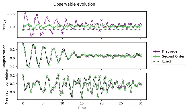
3.4 Ihambing sa eksaktong mga resulta

Ang data sa ibaba ay ang mga precomputed na eksaktong resulta mula sa klasikal na computer.

exact_times = np.array(
    [
        0.0,
        0.3,
        0.6,
        0.8999999999999999,
        1.2,
        1.5,
        1.7999999999999998,
        2.1,
        2.4,
        2.6999999999999997,
        3.0,
        3.3,
        3.5999999999999996,
        3.9,
        4.2,
        4.5,
        4.8,
        5.1,
        5.3999999999999995,
        5.7,
        6.0,
        6.3,
        6.6,
        6.8999999999999995,
        7.199999999999999,
        7.5,
        7.8,
        8.1,
        8.4,
        8.7,
        9.0,
        9.299999999999999,
        9.6,
        9.9,
        10.2,
        10.5,
        10.799999999999999,
        11.1,
        11.4,
        11.7,
        12.0,
        12.299999999999999,
        12.6,
        12.9,
        13.2,
        13.5,
        13.799999999999999,
        14.1,
        14.399999999999999,
        14.7,
        15.0,
        15.299999999999999,
        15.6,
        15.899999999999999,
        16.2,
        16.5,
        16.8,
        17.099999999999998,
        17.4,
        17.7,
        18.0,
        18.3,
        18.599999999999998,
        18.9,
        19.2,
        19.5,
        19.8,
        20.099999999999998,
        20.4,
        20.7,
        21.0,
        21.3,
        21.599999999999998,
        21.9,
        22.2,
        22.5,
        22.8,
        23.099999999999998,
        23.4,
        23.7,
        24.0,
        24.3,
        24.599999999999998,
        24.9,
        25.2,
        25.5,
        25.8,
        26.099999999999998,
        26.4,
        26.7,
        27.0,
        27.3,
        27.599999999999998,
        27.9,
        28.2,
        28.5,
        28.799999999999997,
        29.099999999999998,
        29.4,
        29.7,
        30.0,
    ]
)
exact_energy = np.array(
    [
        -1.1184402376762155,
        -1.1184402376762157,
        -1.1184402376762157,
        -1.1184402376762148,
        -1.1184402376762153,
        -1.1184402376762155,
        -1.1184402376762148,
        -1.118440237676216,
        -1.118440237676216,
        -1.1184402376762166,
        -1.1184402376762148,
        -1.118440237676216,
        -1.1184402376762153,
        -1.1184402376762148,
        -1.118440237676217,
        -1.118440237676215,
        -1.1184402376762161,
        -1.1184402376762157,
        -1.118440237676217,
        -1.1184402376762161,
        -1.1184402376762137,
        -1.1184402376762161,
        -1.1184402376762161,
        -1.118440237676218,
        -1.1184402376762155,
        -1.1184402376762166,
        -1.1184402376762155,
        -1.1184402376762137,
        -1.1184402376762186,
        -1.1184402376762215,
        -1.1184402376762148,
        -1.118440237676216,
        -1.1184402376762166,
        -1.1184402376762148,
        -1.1184402376762121,
        -1.1184402376762166,
        -1.1184402376762181,
        -1.1184402376762137,
        -1.1184402376762148,
        -1.1184402376762193,
        -1.1184402376762108,
        -1.1184402376762144,
        -1.118440237676217,
        -1.1184402376762197,
        -1.1184402376762153,
        -1.1184402376762161,
        -1.1184402376762184,
        -1.1184402376762126,
        -1.118440237676214,
        -1.118440237676214,
        -1.1184402376762161,
        -1.118440237676212,
        -1.1184402376762164,
        -1.118440237676217,
        -1.1184402376762121,
        -1.1184402376762157,
        -1.1184402376762212,
        -1.1184402376762217,
        -1.1184402376762206,
        -1.118440237676222,
        -1.1184402376762166,
        -1.118440237676212,
        -1.1184402376762137,
        -1.11844023767622,
        -1.1184402376762206,
        -1.118440237676219,
        -1.1184402376762153,
        -1.1184402376762164,
        -1.118440237676209,
        -1.1184402376762144,
        -1.1184402376762161,
        -1.118440237676216,
        -1.1184402376762173,
        -1.118440237676214,
        -1.1184402376762093,
        -1.1184402376762184,
        -1.1184402376762126,
        -1.118440237676213,
        -1.1184402376762195,
        -1.1184402376762095,
        -1.1184402376762075,
        -1.1184402376762197,
        -1.1184402376762141,
        -1.1184402376762146,
        -1.1184402376762184,
        -1.118440237676218,
        -1.1184402376762224,
        -1.118440237676219,
        -1.118440237676218,
        -1.1184402376762206,
        -1.1184402376762168,
        -1.118440237676221,
        -1.118440237676218,
        -1.1184402376762148,
        -1.1184402376762106,
        -1.1184402376762173,
        -1.118440237676216,
        -1.118440237676216,
        -1.1184402376762113,
        -1.1184402376762275,
        -1.1184402376762195,
    ]
)
exact_magnetization = np.array(
    [
        0.3333333333333333,
        0.26316769633415005,
        0.0912947227110664,
        -0.09317712543141576,
        -0.20391854332115245,
        -0.19318196655046493,
        -0.06411527074401464,
        0.12558269854206197,
        0.28252754464640606,
        0.3264196194042506,
        0.2361586169847769,
        0.060894367906122224,
        -0.10842387093076275,
        -0.18636359582538073,
        -0.1338364343947887,
        0.020284606520827753,
        0.19151142743926025,
        0.2905341647678381,
        0.2723014646745304,
        0.15147481733047252,
        -0.008179102877790292,
        -0.1242999208732406,
        -0.1372529247781061,
        -0.04083616185958952,
        0.11066094926716476,
        0.23140661570567636,
        0.2587109403786205,
        0.1868237670027325,
        0.061201779383143744,
        -0.051391248969654205,
        -0.09843899603365061,
        -0.061297056158849166,
        0.04199010081939773,
        0.15861461430963147,
        0.22336830674799552,
        0.20179555623336537,
        0.11407111438609417,
        0.01609419104778282,
        -0.04239611796730001,
        -0.04249123521065924,
        0.008850291714888112,
        0.08780898151558082,
        0.1561486776507056,
        0.17627348772811832,
        0.13870676179652253,
        0.07205869195282538,
        0.018300003064909465,
        0.0001095640839572417,
        0.015157929316037586,
        0.05077755280969454,
        0.09245534457650838,
        0.12206907551110702,
        0.12284950557969157,
        0.09570215398601932,
        0.06294378255078983,
        0.045503313813986014,
        0.043389819499542556,
        0.046725117769796744,
        0.054956411358382404,
        0.0713814528253614,
        0.08743689703248492,
        0.08951216359166674,
        0.07878386475305985,
        0.06955669116405788,
        0.06639892435963689,
        0.05890378761746903,
        0.04541796525844558,
        0.0414221088331947,
        0.05499634106912299,
        0.07409418836014572,
        0.08371859070160165,
        0.08211623987959302,
        0.07615055161378328,
        0.06702584458783024,
        0.051891407742740085,
        0.038049378383635625,
        0.03825614149768043,
        0.054183218463525695,
        0.0753534475741016,
        0.08853147112587295,
        0.08767917178542013,
        0.07709383184439536,
        0.06308595032042386,
        0.0498812359204284,
        0.04299040064096167,
        0.04769159891460652,
        0.06483569572288776,
        0.08698035745435016,
        0.10047391641776235,
        0.09747255683203637,
        0.08098863187287358,
        0.05959496723987331,
        0.04383882265040485,
        0.04232138798062125,
        0.05720514169944535,
        0.08201306299870219,
        0.10274898262000469,
        0.10707552455080133,
        0.09210856128265357,
        0.06379922105742579,
        0.03624325103307953,
    ]
)
exact_correlation = np.array(
    [
        0.2,
        0.1247704225763532,
        0.01943938494098705,
        0.03854917181332821,
        0.11196616231067426,
        0.0906546700356683,
        0.01629373561896267,
        0.011352652889791095,
        0.0636185676540077,
        0.09543834437789013,
        0.10058518161011307,
        0.11829217731417431,
        0.1397812224038133,
        0.12316460402216707,
        0.08541383059335775,
        0.06144846844403662,
        0.020246372880505827,
        -0.02693683090021662,
        0.003919250903281282,
        0.1117419430168554,
        0.19676155181256794,
        0.18594408880783336,
        0.1002673802566004,
        0.03821525827438024,
        0.04485205090247377,
        0.05348102743040269,
        0.03160026140008638,
        0.033437649060464834,
        0.10486939975320728,
        0.20249469538955758,
        0.19735507621013149,
        0.0553097261765083,
        -0.04889114490131667,
        0.011685690974970964,
        0.11705971535823065,
        0.11681165998194759,
        0.06637091239560744,
        0.10936684225958895,
        0.20225454101061405,
        0.16284420833341812,
        -0.0025823294931362067,
        -0.0763416631752919,
        0.02985268630418397,
        0.15234468006771007,
        0.14606385406970995,
        0.0935341856492092,
        0.12325421854361143,
        0.17130422930386324,
        0.10383730044042278,
        -0.031333159406547614,
        -0.05241572078596815,
        0.07722509925347705,
        0.17642188574256007,
        0.12765340239966838,
        0.06309968945093776,
        0.11574687130499339,
        0.16978282647206913,
        0.0736143632571229,
        -0.05356602733119409,
        -0.0009649396796768892,
        0.15921620111869142,
        0.17760366431811037,
        0.04736297330213485,
        0.012122870263181897,
        0.13268065586830521,
        0.1728473023503636,
        0.03999259331072221,
        -0.036997053070222885,
        0.06951528580242439,
        0.1769169993516561,
        0.12290448295710298,
        0.012897784654866427,
        0.02859435620982225,
        0.12895847695150875,
        0.13629536955485938,
        0.05394621059822597,
        0.02298040588184324,
        0.07036499900317271,
        0.11706448623132719,
        0.10435285842074606,
        0.055721236329964965,
        0.04676334743672697,
        0.08417924910022263,
        0.10611161955304965,
        0.089304171047322,
        0.06098589533081194,
        0.06314519797488709,
        0.09431492621892917,
        0.09667836915967139,
        0.0651298357290882,
        0.05176966009147416,
        0.06727229484222669,
        0.08871788283607947,
        0.09907054249093444,
        0.09785167773502176,
        0.09277216140054353,
        0.07520999642062785,
        0.05894392248382922,
        0.07236135251622376,
        0.08608284185200156,
        0.07282922961856123,
    ]
)

axes[0].plot(exact_times, exact_energy, c="k", ls=":", label="Exact")
axes[1].plot(exact_times, exact_magnetization, c="k", ls=":", label="Exact")
axes[2].plot(exact_times, exact_correlation, c="k", ls=":", label="Exact")
# Replace the legend
legend.remove()
# Select the labels of only the first axis
legend = fig.legend(
    *axes[0].get_legend_handles_labels(),
    bbox_to_anchor=(1.0, 0.5),
    loc="center left",
    framealpha=0.5,
)
fig.tight_layout()
fig

Output of the previous code cell

4. Pagpapatakbo sa quantum hardware

Susunod, patatakbuhin natin ang time-evolution simulation sa aktwal na quantum hardware. Gagawa tayo ng mas maliit na problema, lattice na may sukat na N=2. Bababaguhin natin ang parameter na $\alpha$ at makikita ang pagkakaiba sa dynamics ng wavefunction.

4.1 Hakbang 1. I-map ang mga klasikal na input sa quantum na problema

Piliin ang paunang mga setting ng simulation:

n_qubits_2 = 2
dt_2 = 1.6
product_formula = LieTrotter(reps=1)

Pagkatapos itakda ang paunang circuit:

Ang paunang spin configuration ay magiging "down-up"

# We prepare an initial state ↓↑ (10).
# Note that Statevector and SparsePauliOp interpret the qubits from right to left
initial_circuit_2 = QuantumCircuit(n_qubits_2)
initial_circuit_2.prepare_state("10")
# Change reps and see the difference when you decompose the circuit
initial_circuit_2.decompose(reps=1).draw("mpl")

Output of the previous code cell

Ngayon kalkulahin ang reference value gamit ang isang ideal statevector simulator.

bar_width = 0.1
# initial_state = Statevector.from_label("10")
final_time = 1.6
eps = 1e-5

# We create the list of angles in radians, with a small epsilon
# the exactly longitudinal field, which would present no dynamics at all
alphas = np.linspace(-np.pi / 2 + eps, np.pi / 2 - eps, 5)

for i, alpha in enumerate(alphas):
    evolved_state_2 = QuantumCircuit(initial_circuit_2.num_qubits)
    evolved_state_2.append(initial_circuit_2, evolved_state_2.qubits)
    hamiltonian_2 = get_hamiltonian(nqubits=2, J=0.2, h=1.0, alpha=alpha)
    single_step_evolution_gates_2 = PauliEvolutionGate(
        hamiltonian_2, dt_2, synthesis=product_formula
    )
    evolved_state_2.append(single_step_evolution_gates_2, evolved_state_2.qubits)
    evolved_state_2 = Statevector(evolved_state_2)
    # Dictionary of probabilities
    amplitudes_dict = evolved_state_2.probabilities_dict()
    labels = list(amplitudes_dict.keys())
    values = list(amplitudes_dict.values())
    # Convert angle to degrees
    alpha_str = f"$\\alpha={int(np.round(alpha * 180 / np.pi))}^\\circ$"
    plt.bar(np.arange(4) + i * bar_width, values, bar_width, label=alpha_str, alpha=0.7)

plt.xticks(np.arange(4) + 2 * bar_width, labels)
plt.xlabel("Measurement")
plt.ylabel("Probability")
plt.suptitle(
    f"Measurement probabilities at $t={final_time}$, for various field angles $\\alpha$\n"
    f"Initial state: 10, Linear lattice of size $L=2$"
)
plt.legend()

<matplotlib.legend.Legend at 0x11c816590>

Output of the previous code cell

Inihanda natin ang isang sistema na ang paunang pagkakasunod-sunod ng mga spin ay $\downarrow\uparrow$ , na katumbas ng $\vert\psi(0)\rangle = \vert10\rangle$ . Pagkatapos itong hayaang mag-evolve ng $t=1.6$ sa ilalim ng isang transversal field ( $\alpha=0^\circ$ ), halos garantisado na masusukat natin ang $\uparrow\downarrow$ , ibig sabihin, magkakaroon ng spin swap. (Tandaan na ang mga label ay binibigyang-kahulugan mula kanan pakaliwa). Kung ang field ay longitudinal ( $\alpha=\pm90^\circ$ ), walang magiging evolution, kaya msusukat natin ang sistema gaya ng dati itong inihanda, $\downarrow\uparrow$ . Sa mga intermediate na anggulo, sa $\alpha=\pm45^\circ$ , maaari tayong masukat ng lahat ng kumbinasyon na may iba't ibang probabilidad, kung saan ang spin swap ang pinakamalamang na mangyari na may probabilidad na 67%.

Bumuo ng circuit para sa HW experiment

circuit_list = []
for i, alpha in enumerate(alphas):
    evolved_state_2 = QuantumCircuit(initial_circuit_2.num_qubits)
    evolved_state_2.append(initial_circuit_2, evolved_state_2.qubits)
    hamiltonian_2 = get_hamiltonian(nqubits=2, J=0.2, h=1.0, alpha=alpha)
    single_step_evolution_gates_2 = PauliEvolutionGate(
        hamiltonian_2, dt_2, synthesis=product_formula
    )
    evolved_state_2.append(single_step_evolution_gates_2, evolved_state_2.qubits)
    evolved_state_2.measure_all()
    circuit_list.append(evolved_state_2)

4.2 Hakbang 2. I-optimize para sa target na hardware

Tukuyin ang isang backend.

service = QiskitRuntimeService()
backend = service.least_busy(operational=True, simulator=False)
backend.name

'ibm_strasbourg'

Pagkatapos i-transpile ang circuit para sa napiling backend.

pm = generate_preset_pass_manager(backend=backend, optimization_level=3)
circuit_isa = pm.run(circuit_list)

Tingnan ang circuit.

circuit_isa[1].draw("mpl", idle_wires=False)

Output of the previous code cell

4.3 Hakbang 3. Isagawa gamit ang mga Qiskit Runtime primitive

Ang Sampler (V2) primitive ng Qiskit ay nagbibigay ng mga bilang ng mga nasukat na bitstring.

sampler = SamplerV2(mode=backend)
job = sampler.run(circuit_isa)
job_id = job.job_id()
print("job id:", job_id)

job id: d13pswfmya70008ek070

I-save ang mga resulta

results = job.result()

4.4 Hakbang 4. Post-process ng mga resulta

Buuin ang histogram ng mga bitstring, na katumbas ng pagsusuri ng wavefunction, at ikumpara ito sa mga ideal na halaga na ipinakita sa itaas.

list_temp = ["00", "01", "10", "11"]

for i, alpha in enumerate(alphas):
    # Dictionary of probabilities
    amplitudes_dict = results[i].data.meas.get_counts()
    values = []
    for str_temp in list_temp:
        values.append(
            amplitudes_dict[str_temp] / 4096.0
        )  # divided by default number of shots
    # Convert angle to degrees
    alpha_str = f"$\\alpha={int(np.round(alpha * 180 / np.pi))}^\\circ$"
    plt.bar(np.arange(4) + i * bar_width, values, bar_width, label=alpha_str, alpha=0.7)

plt.xticks(np.arange(4) + 2 * bar_width, labels)
plt.xlabel("Measurement")
plt.ylabel("Probabilities")
plt.suptitle(
    f"Measurement probabilities at $t={final_time}$, for various field angles $\\alpha$\n"
    f"Initial state: 10, Linear lattice of size $L=2$"
)
plt.legend()

<matplotlib.legend.Legend at 0x11d7af990>

Output of the previous code cell

Nagpapakita tayo rito ng isang halimbawa ng pagbuo ng circuit gamit ang mas mataas na order na (ikaapat na order) Suzuki–Trotter. Subukan nating bumuo ng circuit simulation gamit ang ikaapat na order na Suzuki–Trotter ayon sa mga halimbawang ipinakita sa itaas.

Ang ikaapat na order na Suzuki–Trotter ay maaaring gamitin sa Qiskit sa pamamagitan ng SuzukiTrotter class. Ang ikaapat na order ay maaaring kalkulahin gamit ang sumusunod na recursion relation. Tandaan na ang order ng Suzuki–Trotter ay tinutukoy bilang "2k" sa mga sumusunod na equation.

\hat{U}_{ST(2k)}\left(t\right) = \left[ \hat{U}_{ST(2k-2)}\left(p_k t\right) \right]^2 \hat{U}_{ST(2k-2)}\left( (1- 4 p_k) t\right)\left[ \hat{U}_{ST(2k-2)}\left(p_k t\right) \right]^2

p_k = 1 / \left(4-4^{\frac{1}{2k-1}}\right)

Bumuo ng circuit para sa isang time step

Gamitin ang product_formula_st4 (SuzukiTrotter(order=4)) at bumuo ng circuit para sa isang time step gamit ang ikaapat na order na Suzuki–Trotter. Gayundin, bilangin ang bilang ng mga gate at depth ng circuit at ikumpara ito sa Lie–Trotter at pangalawang order na Suzuki–Trotter.

# Modify the line below (Use PauliEvolutionGate)
single_step_evolution_gates_st4 = PauliEvolutionGate(
    hamiltonian, dt, synthesis=product_formula_st4
)
single_step_evolution_st4 = QuantumCircuit(n_qubits)
single_step_evolution_st4.append(
    single_step_evolution_gates_st4, single_step_evolution_st4.qubits
)
# Let us print some stats
print(
    f"""
Trotter step with second-order Suzuki-Trotter
-----------------------------
Depth: {single_step_evolution_st4.decompose(reps=3).depth()}
Gate count: {len(single_step_evolution_st4.decompose(reps=3))}
Nonlocal gate count: {single_step_evolution_st4.decompose(reps=3).num_nonlocal_gates()}
Gate breakdown: {", ".join([f"{k.upper()}: {v}" for k, v in single_step_evolution_st4.decompose(reps=3).count_ops().items()])}
"""
)
single_step_evolution_st4.decompose(reps=2).draw("mpl", fold=-1)

Trotter step with second-order Suzuki-Trotter
-----------------------------
Depth: 170
Gate count: 265
Nonlocal gate count: 100
Gate breakdown: U3: 115, CX: 100, U1: 50

Output of the previous code cell

# Check Qiskit version
import qiskit

qiskit.__version__

'2.0.2'

1. Panimula​

1.1 Mga Kinakailangan​

1.2 I-import ang mga library​

2. Pag-map ng iyong problema​

2.1 Pagtukoy sa transverse-field Ising Hamiltonian​

Tukuyin ang Hamiltonian​

2.2 Itakda ang mga parameter ng time-evolution simulation​

2.3 Ihanda ang quantum circuit 1 (Paunang estado)​

2.4 Ihanda ang quantum circuit 2 (Iisang circuit para sa time evolution)​

2.5 Itakda ang mga operator na susukatin​

2.6 Isagawa ang time-evolution simulation​

2.7 I-plot ang time evolution ng mga observable​

3. Ehersisyo 1. Magsagawa ng simulation gamit ang second-order Suzuki–Trotter​

3.1 Bumuo ng circuit para sa isang time step​

3.2 Magsagawa ng time-evolution simulation​

3.3 I-plot ang mga resulta ng second-order Suzuki–Trotter​

3.4 Ihambing sa eksaktong mga resulta​

4. Pagpapatakbo sa quantum hardware​

4.1 Hakbang 1. I-map ang mga klasikal na input sa quantum na problema​

Bumuo ng circuit para sa HW experiment​

4.2 Hakbang 2. I-optimize para sa target na hardware​

4.3 Hakbang 3. Isagawa gamit ang mga Qiskit Runtime primitive​

4.4 Hakbang 4. Post-process ng mga resulta​

Bumuo ng circuit para sa isang time step​

1. Panimula

1.1 Mga Kinakailangan

1.2 I-import ang mga library

2. Pag-map ng iyong problema

2.1 Pagtukoy sa transverse-field Ising Hamiltonian

Tukuyin ang Hamiltonian

2.2 Itakda ang mga parameter ng time-evolution simulation

2.3 Ihanda ang quantum circuit 1 (Paunang estado)

2.4 Ihanda ang quantum circuit 2 (Iisang circuit para sa time evolution)

2.5 Itakda ang mga operator na susukatin

2.6 Isagawa ang time-evolution simulation

2.7 I-plot ang time evolution ng mga observable

3. Ehersisyo 1. Magsagawa ng simulation gamit ang second-order Suzuki–Trotter

3.1 Bumuo ng circuit para sa isang time step

3.2 Magsagawa ng time-evolution simulation

3.3 I-plot ang mga resulta ng second-order Suzuki–Trotter

3.4 Ihambing sa eksaktong mga resulta

4. Pagpapatakbo sa quantum hardware

4.1 Hakbang 1. I-map ang mga klasikal na input sa quantum na problema

Bumuo ng circuit para sa HW experiment

4.2 Hakbang 2. I-optimize para sa target na hardware

4.3 Hakbang 3. Isagawa gamit ang mga Qiskit Runtime primitive

4.4 Hakbang 4. Post-process ng mga resulta

Bumuo ng circuit para sa isang time step