Panimula sa Qiskit AI-powered transpiler
Tinatayang paggamit: 5 minuto sa IBM Heron (TANDAAN: Tantiya lamang ito. Maaaring mag-iba ang iyong runtime.)
Mga layunin sa pagkatuto
Pagkatapos ng tutorial na ito, dapat maunawaan ng mga user ang:
- Kung paano gamitin ang AI-powered transpiler (
generate_ai_pass_manager) bilang direktang kapalit ng standard na transpiler - Kung paano inihahambing ang AI-powered transpiler sa default na transpiler sa mga tuntunin ng two-qubit depth, gate count, at transpilation time
- Kung paano gamitin ang mirror circuits upang suriin ang kalidad ng transpilation sa pamamagitan ng hardware execution
Mga kinakailangan
Iminumungkahi naming pamilyar ang mga user sa mga sumusunod na paksa bago dumaan sa tutorial na ito:
Background
Ang Qiskit AI-powered transpiler ay nagpapakilala ng mga transpilation pass na batay sa machine learning na maaaring gumawa ng mas maikli at mas hardware-efficient na mga circuit kaysa sa tradisyonal na heuristic na mga pamamaraan tulad ng SABRE. Ang mas maikling mga circuit ay nag-iipon ng mas kaunting ingay, na direktang nagpapabuti ng kalidad ng resulta sa tunay na quantum hardware.
Sa tutorial na ito, inihahambing natin ang dalawang estratehiya ng transpilation:
| Estratehiya | API |
|---|---|
| Default | generate_preset_pass_manager(optimization_level=3, ...) |
| AI | generate_ai_pass_manager(optimization_level=1, ai_optimization_level=3, ...) |
Sinusukat natin ang tatlong metric para sa bawat estratehiya: two-qubit gate depth, kabuuang gate count, at transpilation runtime.
Mga benchmark ng AI-powered transpiler
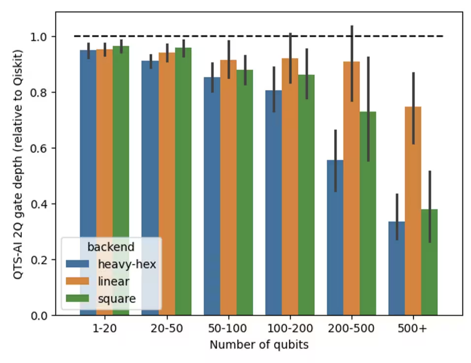
Sa mga benchmarking test, ang AI-powered transpiler ay patuloy na gumawa ng mas mababaw at mas mataas na kalidad na mga circuit kumpara sa standard na Qiskit transpiler. Para sa mga test na ito, ginamit namin ang default pass manager strategy ng Qiskit, na naka-configure sa generate_preset_pass_manager. Bagama't ang default strategy na ito ay madalas na epektibo, maaari itong mahirapan sa mas malalaki o mas kumplikadong mga circuit. Sa kabaligtaran, ang mga AI-powered pass ay nakamit ang average na 24% reduction sa two-qubit gate counts at 36% reduction sa circuit depth para sa malalaking circuit (100+ qubits) kapag nag-transpile sa heavy-hex topology ng IBM Quantum® hardware. Para sa higit pang impormasyon tungkol sa mga benchmark na ito, sumangguni sa blog na ito.
Sinusuri ng tutorial na ito ang mga pangunahing benepisyo ng AI passes at kung paano ito inihahambing sa tradisyonal na mga pamamaraan.
Mga kinakailangan
Bago simulan ang tutorial na ito, siguraduhing mayroon kayong sumusunod na naka-install:
- Qiskit SDK v2.0 o mas bago, na may visualization support
- Qiskit Runtime (
pip install qiskit-ibm-runtime) v0.22 o mas bago - Qiskit IBM Transpiler with AI local mode (
pip install 'qiskit-ibm-transpiler[ai-local-mode]') - Qiskit Aer (
pip install qiskit-aer)
Setup
# Added by doQumentation — required packages for this notebook
!pip install -q matplotlib qiskit qiskit-aer qiskit-ibm-runtime qiskit-ibm-transpiler
from qiskit import QuantumCircuit
from qiskit.circuit.random import random_circuit
from qiskit.transpiler import generate_preset_pass_manager
from qiskit_ibm_runtime import QiskitRuntimeService, SamplerV2
from qiskit_ibm_transpiler import generate_ai_pass_manager
from qiskit_aer import AerSimulator
from qiskit_aer.noise import NoiseModel, depolarizing_error
import matplotlib.pyplot as plt
from statistics import mean, stdev
import time
import logging

seed = 42

def transpile_with_metrics(pass_manager, circuit):
    """Transpile a circuit and return the result along with key metrics."""
    start = time.time()
    qc_out = pass_manager.run(circuit)
    elapsed = time.time() - start

    depth_2q = qc_out.depth(lambda x: x.operation.num_qubits == 2)
    gate_count = qc_out.size()

    return qc_out, {
        "depth_2q": depth_2q,
        "gate_count": gate_count,
        "time_s": round(elapsed, 3),
    }

def remap_to_contiguous(tqc):
    """Remap a transpiled circuit to use contiguous qubit indices.

    Transpiled circuits target specific physical qubits (e.g., qubit 45, 67)
    on a large backend. This remaps them to 0, 1, 2, ... so Aer only
    simulates the active qubits."""
    active = sorted(
        {tqc.find_bit(q).index for inst in tqc.data for q in inst.qubits}
    )
    qubit_map = {old: new for new, old in enumerate(active)}
    new_qc = QuantumCircuit(len(active))
    for inst in tqc.data:
        old_indices = [tqc.find_bit(q).index for q in inst.qubits]
        new_qc.append(inst.operation, [qubit_map[i] for i in old_indices])
    return new_qc

def build_mirror_circuit(tqc, simulate=True):
    """Build a mirror circuit: U followed by U-dagger, with measurements.

    The expected output is always |0...0>, so measuring the survival
    probability reveals how much noise each transpilation strategy adds.

    Args:
        tqc: A transpiled circuit.
        simulate: If True (default), remap to contiguous qubits so Aer
            only simulates the active qubits. If False, keep the full
            physical layout for hardware execution."""
    if simulate:
        tqc = remap_to_contiguous(tqc)
    mirror = tqc.compose(tqc.inverse())
    mirror.measure_all()
    return mirror

def print_summary(results):
    """Print a summary of each metric as mean +/- stdev across all circuits,
    along with the mean percentage improvement of AI over Default."""
    metrics = [
        ("Depth 2Q", "Depth 2Q (Default)", "Depth 2Q (AI)"),
        ("Gate Count", "Gate Count (Default)", "Gate Count (AI)"),
        ("Time (s)", "Time (Default)", "Time (AI)"),
    ]
    header = (
        f"{'Metric':<12}{'Default (mean +/- std)':>24}"
        f"{'AI (mean +/- std)':>22}{'AI % improvement':>22}"
    )
    print(header)
    print("-" * len(header))
    for label, col_def, col_ai in metrics:
        defaults = [r[col_def] for r in results]
        ais = [r[col_ai] for r in results]
        pct = [(d - a) / d * 100 for d, a in zip(defaults, ais)]
        default_str = f"{mean(defaults):.1f} +/- {stdev(defaults):.1f}"
        ai_str = f"{mean(ais):.1f} +/- {stdev(ais):.1f}"
        pct_str = f"{mean(pct):+.1f}% +/- {stdev(pct):.1f}%"
        print(f"{label:<12}{default_str:>24}{ai_str:>22}{pct_str:>22}")

def plot_metrics_and_pct(results, title_prefix):
    """Plot metric comparisons and percentage improvement of AI over Default."""
    qubits = [r["Qubits"] for r in results]
    metrics = [
        ("Depth 2Q (Default)", "Depth 2Q (AI)", "Two-Qubit Depth"),
        ("Gate Count (Default)", "Gate Count (AI)", "Gate Count"),
        ("Time (Default)", "Time (AI)", "Transpilation Time"),
    ]

    # Row 1: raw metric comparison
    fig, axs = plt.subplots(1, 3, figsize=(21, 5))
    fig.suptitle(
        f"{title_prefix}: Metric Comparison",
        fontsize=15,
        fontweight="bold",
        y=1.02,
    )
    for ax, (col_def, col_ai, label) in zip(axs, metrics):
        ax.plot(qubits, [r[col_def] for r in results], "o-", label="Default")
        ax.plot(qubits, [r[col_ai] for r in results], "s-", label="AI")
        ax.set_title(label)
        ax.set_xlabel("Number of Qubits")
        ax.set_ylabel(label)
        ax.legend()
    plt.tight_layout()
    plt.show()

    # Row 2: percentage improvement
    fig, axs = plt.subplots(1, 3, figsize=(21, 5))
    fig.suptitle(
        f"{title_prefix}: % Improvement of AI over Default",
        fontsize=15,
        fontweight="bold",
        y=1.02,
    )
    for ax, (col_def, col_ai, label) in zip(axs, metrics):
        pct = [(r[col_def] - r[col_ai]) / r[col_def] * 100 for r in results]
        ax.axhline(
            0, color="#1f77b4", linewidth=2, label="Default (baseline)"
        )
        ax.plot(qubits, pct, "s-", color="#ff7f0e", label="AI")
        ax.fill_between(qubits, 0, pct, alpha=0.15, color="#ff7f0e")
        ax.set_title(label)
        ax.set_xlabel("Number of Qubits")
        ax.set_ylabel("% Improvement")
        ax.legend()
    plt.tight_layout()
    plt.show()

# Suppress verbose AI-powered transpiler logs
logging.getLogger(
    "qiskit_ibm_transpiler.wrappers.ai_local_synthesis"
).setLevel(logging.WARNING)
Halimbawa sa maliit na sukat na simulator
Hakbang 1: I-map ang mga klasikal na input sa isang quantum na problema
Bumubuo tayo ng 20 random na circuit na may depth na 4, kung saan ang bilang ng qubits ay mula anim hanggang 25. Ang mga circuit na ito ang magiging mga test case natin para sa paghahambing ng mga estratehiya ng transpilation.
num_circuits_sim = 20
depth_sim = 4
qubit_range_sim = list(range(6, 26))

circuits_sim = [
    # We have only two qubit gates, as those test how well the transpiler can optimize the circuit.
    random_circuit(
        num_qubits=n,
        depth=depth_sim,
        max_operands=2,
        num_operand_distribution={2: 1},
        seed=seed + i,
    )
    for i, n in enumerate(qubit_range_sim)
]

print(
    f"Created {len(circuits_sim)} circuits with qubit counts: {qubit_range_sim}"
)
circuits_sim[0].draw(output="mpl", fold=-1)
Created 20 circuits with qubit counts: [6, 7, 8, 9, 10, 11, 12, 13, 14, 15, 16, 17, 18, 19, 20, 21, 22, 23, 24, 25]

Hakbang 2: I-optimize ang problema para sa quantum hardware execution
Binubuo natin ang default na (SABRE) pass manager para sa piniling backend. Parehong estratehiya ng transpilation ay nagta-target sa buong coupling map ng backend. Ang lokal na simulation sa ibang pagkakataon ay nananatiling tractable dahil ang hakbang ng simulation ay gumagamit ng remap_to_contiguous upang muling i-label ang bawat transpiled na circuit sa mga aktibong qubit lamang nito, kaya ang Aer ay nagsi-simulate lamang ng mga qubits na iyon sa halip na ang buong device.
service = QiskitRuntimeService()
backend = service.least_busy(
    min_num_qubits=100, operational=True, simulator=False
)

pm_default_sim = generate_preset_pass_manager(
    optimization_level=3,
    backend=backend,
    seed_transpiler=seed,
)
results_sim = []

for i, qc in enumerate(circuits_sim):
    n = qubit_range_sim[i]

    qc_default, m_default = transpile_with_metrics(pm_default_sim, qc)

    # Create a fresh AI pass manager each iteration to avoid stale layout state
    pm_ai = generate_ai_pass_manager(
        optimization_level=1,
        ai_optimization_level=3,
        backend=backend,
    )
    qc_ai, m_ai = transpile_with_metrics(pm_ai, qc)

    results_sim.append(
        {
            "Qubits": n,
            "Depth 2Q (Default)": m_default["depth_2q"],
            "Depth 2Q (AI)": m_ai["depth_2q"],
            "Gate Count (Default)": m_default["gate_count"],
            "Gate Count (AI)": m_ai["gate_count"],
            "Time (Default)": m_default["time_s"],
            "Time (AI)": m_ai["time_s"],
        }
    )

print_summary(results_sim)
Fetching 4 files: 0%| | 0/4 [00:00<?, ?it/s]
Metric        Default (mean +/- std)     AI (mean +/- std)      AI % improvement
--------------------------------------------------------------------------------
Depth 2Q               33.0 +/- 12.9          26.4 +/- 8.0      +15.8% +/- 17.6%
Gate Count           522.0 +/- 266.0       560.5 +/- 279.1        -9.0% +/- 9.0%
Time (s)                 0.0 +/- 0.0           0.2 +/- 0.1    -893.6% +/- 362.9%
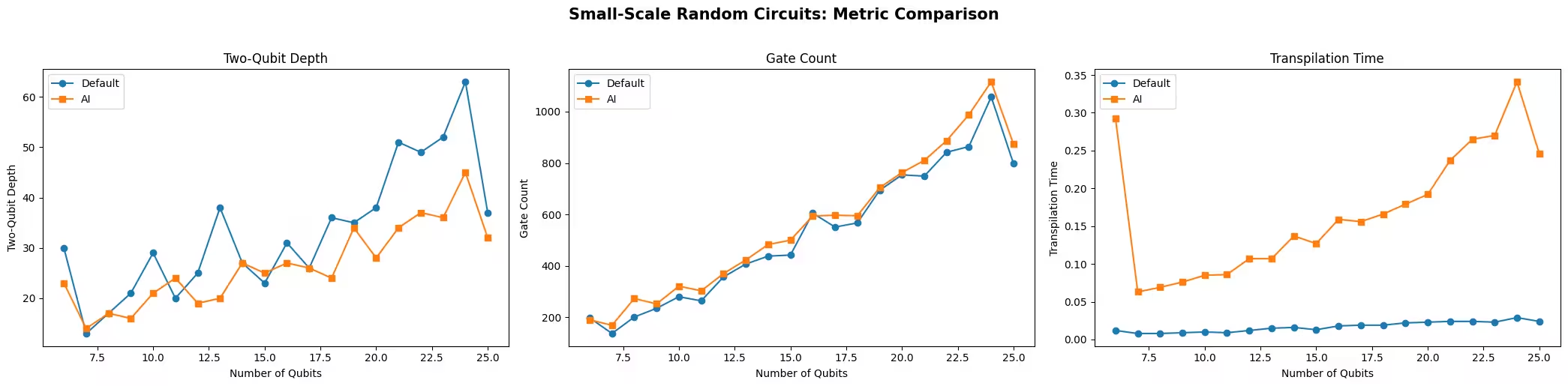
Ipinapakita ng summary table ang mean at standard deviation ng bawat metric sa lahat ng 20 circuit, kasama ang average na porsyento ng pagpapabuti ng AI-powered transpiler kumpara sa default. Ang mga positibong halaga ay nagpapahiwatig na ang AI-powered transpiler ay gumawa ng mas magandang mga resulta; ang mga negatibong halaga ay nagpapahiwatig na ang default ay mas maganda.
Para sa maliit na sukat na halimbawang ito, ang AI-powered transpiler ay nakakamit ng halos 16% na mas mababang two-qubit depth sa average, ngunit sa gastos ng halos 9% na mas mataas na gate count. Binibigyang-diin nito ang isang mahalagang trade-off kapag pumipili sa pagitan ng dalawang estratehiya: ang AI-powered transpiler ay inuuna ang pagbabawas ng depth (mas kaunting magkakasunod na layer ng two-qubit gates), habang ang default na transpiler (SABRE) ay inuuna ang pagpapaliit ng kabuuang gate count (mas kaunting SWAP insertions). Depende sa iyong application, ang isang metric ay maaaring mas mahalaga kaysa sa isa pa.
plot_metrics_and_pct(results_sim, "Small-Scale Random Circuits")
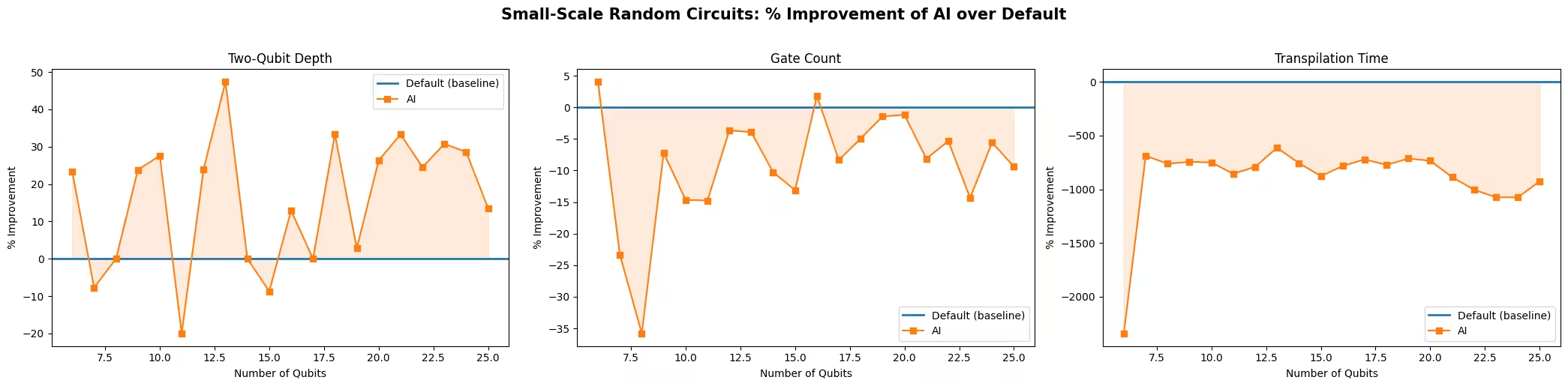
Two-qubit depth: Ang AI-powered transpiler ay karaniwang gumagawa ng mga circuit na may mas mababang two-qubit depth. Ang depth ay isa sa mga pangunahing metric na sinanay ang AI routing model na i-optimize, at ang pagpapabuti ay makikita sa karamihan ng mga laki ng circuit, bagama't ang SABRE ay makapantay o makahigit dito sa mga indibidwal na circuit.
Gate count: Ang mga resulta ay malapit na magkatulad sa sukat na ito, kung saan ang SABRE ay may bahagyang kalamangan sa kabuuan. Ang routing heuristic ng SABRE ay idinisenyo upang mabawasan ang bilang ng mga inilagay na SWAP gate, na direktang nagbabawas ng gate count. Sa maliliit na laki ng circuit, maliit ang pagkakaiba.
Transpilation time: Ang runtime ng SABRE ay halos pare-pareho anuman ang bilang ng qubit, kaya ang laki ng circuit ay may maliit na epekto sa transpilation time nito sa sukat na ito. Ang core routing logic ng SABRE ay lubos na na-optimize (higit na isinagawa sa Rust). Ang AI-powered transpiler ay tumatagal nang mas matagal at nagsa-scale ayon sa laki ng circuit, bagama't ang mga ganap na oras ay nananatiling makatwirang angkop para sa interactive na paggamit.
Hakbang 3: Isagawa gamit ang Qiskit primitives
Upang masuri ang epekto ng transpilation sa circuit fidelity, bumuo ng mga mirror circuit mula sa 10-qubit na kaso at patakbuhin ang mga ito sa Aer simulator na may simpleng noise model. Ang inaasahang output ng isang mirror circuit ay palaging ang all-zeros bitstring, kaya ang posibilidad ng pagsukat ng ay nagpapakita kung gaano kahusay na pinapanatili ng bawat estratehiya ng transpilation ang fidelity.
# Use the 10-qubit circuit (index where qubits == 10)
idx_10q = qubit_range_sim.index(10)

qc_10q = circuits_sim[idx_10q]
qc_default_10q, _ = transpile_with_metrics(pm_default_sim, qc_10q)

pm_ai = generate_ai_pass_manager(
    optimization_level=1,
    ai_optimization_level=3,
    backend=backend,
)
qc_ai_10q, _ = transpile_with_metrics(pm_ai, qc_10q)

tqc_methods = {
    "Default": qc_default_10q,
    "AI": qc_ai_10q,
}

print(
    f"Default: depth {qc_default_10q.depth()}, gates {qc_default_10q.size()}"
)
print(f"AI:      depth {qc_ai_10q.depth()}, gates {qc_ai_10q.size()}")
Default: depth 84, gates 280
AI:      depth 91, gates 343
# Build a simple depolarizing noise model
noise_model = NoiseModel()
noise_model.add_all_qubit_quantum_error(
    depolarizing_error(0.001, 1),
    ["sx", "x", "rz"],  # ~0.1% per 1Q gate
)
noise_model.add_all_qubit_quantum_error(
    depolarizing_error(0.01, 2),
    ["cx", "ecr"],  # ~1% per 2Q gate
)

aer_sim = AerSimulator(noise_model=noise_model)

shots = 10000
survival_probs = {}

for method, tqc in tqc_methods.items():
    mirror = build_mirror_circuit(tqc, simulate=True)

    sampler = SamplerV2(mode=aer_sim)
    job = sampler.run([mirror], shots=shots)
    counts = job.result()[0].data.meas.get_counts()

    all_zeros = "0" * mirror.num_qubits
    survival = counts.get(all_zeros, 0) / shots
    survival_probs[method] = survival
    print(
        f"{method:8s}  P(|00...0>) = {survival:.4f}  ({counts.get(all_zeros, 0)}/{shots})"
    )
Default   P(|00...0>) = 0.8460  (8460/10000)
AI        P(|00...0>) = 0.8121  (8121/10000)
Pinatakbo namin ang parehong mirror circuit sa pamamagitan ng Aer simulator na may simpleng depolarizing noise model. Ang survival probability, na tinukoy bilang porsyento ng mga shot na nagbabalik ng all-zeros bitstring, ay nagsusukat ng dami ng ingay na idinagdag ng bawat estratehiya ng transpilation.
Hakbang 4: I-post-process at ibalik ang resulta sa nais na klasikal na format
Kinukuha natin ang posibilidad ng pagsukat ng all-zeros bitstring mula sa parehong mga run. Ang mas mataas na survival probability ay nagpapahiwatig ng mas magandang fidelity, ibig sabihin ang transpilation ay nagdagdag ng mas kaunting ingay. Ang plot sa ibaba ay nagpapakita ng complement, 1 - P(|0...0>), upang ang mas mababang bar ay nagpapahiwatig ng mas magandang fidelity at ang maliliit na pagkakaiba sa error ay mas madaling makita.
# Plot 1 - P(|0...0>), the probability of an erroneous (non-zero) outcome.
# A lower bar means the transpilation introduced less noise.
error_probs = {method: 1 - p for method, p in survival_probs.items()}

fig, ax = plt.subplots(figsize=(6, 4))
ax.bar(
    error_probs.keys(),
    error_probs.values(),
    color=["steelblue", "coral"],
)
ax.set_ylabel("1 - P(|0...0>)")
ax.set_title("Mirror Circuit Error (10-qubit, Aer Simulator)")
ax.set_ylim(0, 1)
plt.tight_layout()
plt.show()

Sa kasong ito, ang default na transpiler ay gumawa ng parehong mas mababaw at mas maliit na circuit para sa partikular na 10-qubit na instansyang ito, kaya ang mas mataas na fidelity nito ay inaasahan. Ang mga resulta bawat circuit ay nag-iiba: tulad ng ipinapakita ng summary table sa itaas, ang kalamangan ng AI-powered transpiler ay nasa mas mababang two-qubit depth sa average, hindi sa bawat indibidwal na circuit. Kung aling estratehiya ang magbubunga ng mas mataas na fidelity ay nakasalalay sa kalikasan ng pagkakaiba sa bawat metric, ang mga katangian ng ingay ng hardware, at ang istruktura ng circuit. Sa ilalim ng isang pare-parehong depolarizing noise model, ang kabuuang gate count ay madalas na may mas direktang epekto sa naipon na error kaysa sa depth lamang.
Halimbawa sa malalaking sukat na hardware
Mga Hakbang 1-4
Dito ang lahat ng mga detalyeng ito ay pinagsama sa isang malinaw na workflow sa mas malaking sukat, na pagkatapos ay pinapatakbo sa tunay na quantum hardware.
Ang code sa ibaba ay bumubuo ng 25 random na circuit na may depth na 8, kung saan ang bilang ng qubits ay mula 26 hanggang 50. Ang mga circuit na ito ay pagkatapos ay tina-transpile sa parehong estratehiya at kinokolekta ang parehong mga metric. Pagkatapos ay bumubuo tayo ng mga mirror circuit mula sa 26-qubit na kaso at isinusumite ang mga ito sa tunay na backend.
# -------------------------Step 1-------------------------
num_circuits_hw = 25
depth_hw = 8
qubit_range_hw = list(range(26, 51))

circuits_hw = [
    # We have only two qubit gates, as those test how well the transpiler can optimize the circuit.
    random_circuit(
        num_qubits=n,
        depth=depth_hw,
        max_operands=2,
        num_operand_distribution={2: 1},
        seed=seed + i,
    )
    for i, n in enumerate(qubit_range_hw)
]

print(
    f"Created {len(circuits_hw)} circuits with qubit counts: {qubit_range_hw}"
)
Created 25 circuits with qubit counts: [26, 27, 28, 29, 30, 31, 32, 33, 34, 35, 36, 37, 38, 39, 40, 41, 42, 43, 44, 45, 46, 47, 48, 49, 50]
# -------------------------Step 2-------------------------
pm_default = generate_preset_pass_manager(
    optimization_level=3,
    backend=backend,
    seed_transpiler=seed,
)

results_hw = []

for i, qc in enumerate(circuits_hw):
    n = qubit_range_hw[i]

    qc_default, m_default = transpile_with_metrics(pm_default, qc)

    # Create a fresh AI pass manager each iteration to avoid stale layout state
    pm_ai = generate_ai_pass_manager(
        optimization_level=1,
        ai_optimization_level=3,
        backend=backend,
    )
    qc_ai, m_ai = transpile_with_metrics(pm_ai, qc)

    results_hw.append(
        {
            "Qubits": n,
            "Depth 2Q (Default)": m_default["depth_2q"],
            "Depth 2Q (AI)": m_ai["depth_2q"],
            "Gate Count (Default)": m_default["gate_count"],
            "Gate Count (AI)": m_ai["gate_count"],
            "Time (Default)": m_default["time_s"],
            "Time (AI)": m_ai["time_s"],
        }
    )

print_summary(results_hw)
Metric        Default (mean +/- std)     AI (mean +/- std)      AI % improvement
--------------------------------------------------------------------------------
Depth 2Q              217.4 +/- 50.4        191.0 +/- 35.6      +10.9% +/- 10.7%
Gate Count         4513.3 +/- 1394.3     5227.1 +/- 1536.4       -16.4% +/- 5.8%
Time (s)                 0.1 +/- 0.0           3.5 +/- 1.5   -3588.2% +/- 643.6%
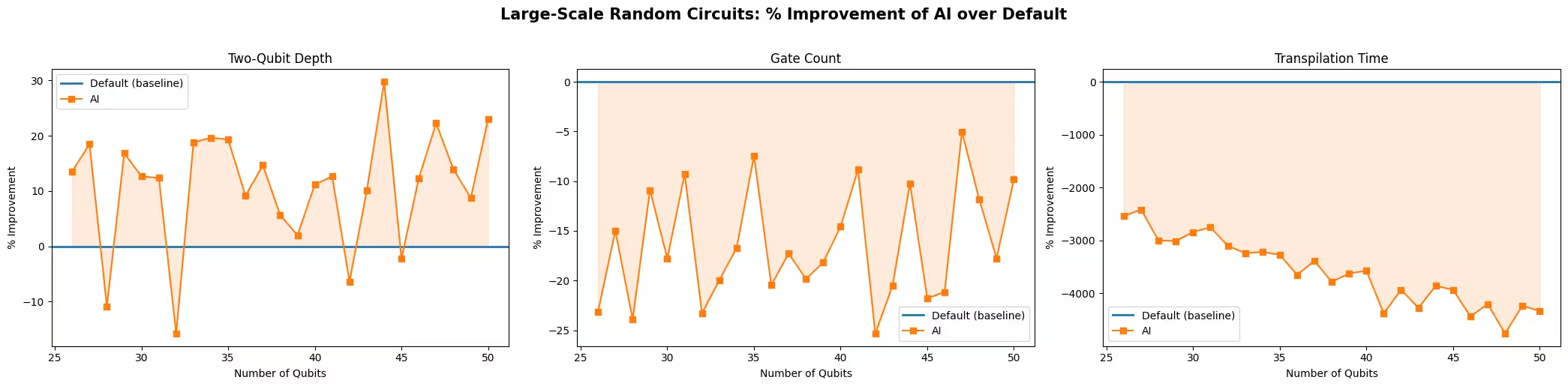
plot_metrics_and_pct(results_hw, "Large-Scale Random Circuits")
# -------------------------Step 3-------------------------
# Build mirror circuits from the 26-qubit case
idx_26q = qubit_range_hw.index(26)

qc_26q = circuits_hw[idx_26q]
qc_default_26q, _ = transpile_with_metrics(pm_default, qc_26q)

pm_ai = generate_ai_pass_manager(
    optimization_level=1,
    ai_optimization_level=3,
    backend=backend,
)
qc_ai_26q, _ = transpile_with_metrics(pm_ai, qc_26q)

mirror_default_hw = build_mirror_circuit(qc_default_26q, simulate=False)
mirror_ai_hw = build_mirror_circuit(qc_ai_26q, simulate=False)

# Re-transpile to basis gates (the inverse can introduce gates like sxdg)
pm_basis = generate_preset_pass_manager(
    optimization_level=0,
    backend=backend,
)
mirror_default_hw = pm_basis.run(mirror_default_hw)
mirror_ai_hw = pm_basis.run(mirror_ai_hw)

print(
    f"Mirror circuit (Default): depth {mirror_default_hw.depth()}, gates {mirror_default_hw.size()}"
)
print(
    f"Mirror circuit (AI):      depth {mirror_ai_hw.depth()}, gates {mirror_ai_hw.size()}"
)

# Submit to real hardware
sampler_hw = SamplerV2(mode=backend)
sampler_hw.options.environment.job_tags = ["TUT_AITI"]

shots_hw = 500000
job_hw = sampler_hw.run([mirror_default_hw, mirror_ai_hw], shots=shots_hw)
print(f"Job submitted: {job_hw.job_id()}")
Mirror circuit (Default): depth 1577, gates 9672
Mirror circuit (AI):      depth 1235, gates 11092
Job submitted: d8gt7vm6983c73dqbg0g
# -------------------------Step 4-------------------------
result_hw = job_hw.result()

survival_probs_hw = {}
for i, method in enumerate(["Default", "AI"]):
    counts = result_hw[i].data.meas.get_counts()
    mirror = [mirror_default_hw, mirror_ai_hw][i]
    all_zeros = "0" * mirror.num_qubits
    survival = counts.get(all_zeros, 0) / shots_hw
    survival_probs_hw[method] = survival
    print(
        f"{method:8s}  P(|00...0>) = {survival:.4f}  ({counts.get(all_zeros, 0)}/{shots_hw})"
    )

# Plot 1 - P(|0...0>), the probability of an erroneous (non-zero) outcome.
# A lower bar means the transpilation introduced less noise.
error_probs_hw = {method: 1 - p for method, p in survival_probs_hw.items()}

fig, ax = plt.subplots(figsize=(6, 4))
ax.bar(
    error_probs_hw.keys(),
    error_probs_hw.values(),
    color=["steelblue", "coral"],
)
ax.set_ylabel("1 - P(|0...0>)")
ax.set_title(f"Mirror Circuit Error (26-qubit, {backend.name})")
ax.set_ylim(0, 1)
plt.tight_layout()
plt.show()
Default   P(|00...0>) = 0.0005  (239/500000)
AI        P(|00...0>) = 0.0050  (2516/500000)

Pagsusuri ng mga resulta
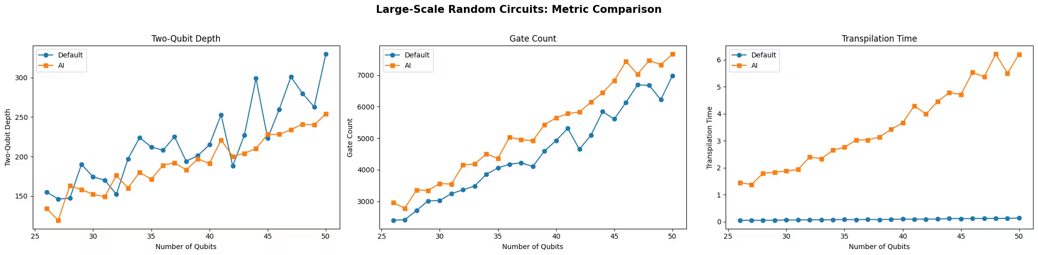
Pinapalakas ng malalaking-sukat na mga resulta ang mga trend na naobserbahan sa maliit na sukat na halimbawa, ngayon sa mas demanding na sukat.
Two-qubit depth: Ang AI-powered transpiler ay patuloy na naghahatid ng kapansin-pansing mas mababang two-qubit depth sa buong hanay ng mga laki ng circuit. Ang depth optimization ay isa sa mga pangunahing layunin na sinanay ang AI routing model, at ang kalamangan ay mas kapansin-pansin sa mas malalaking bilang ng qubit kung saan ang routing problem ay nagiging mas mahirap para sa mga heuristic na pamamaraan.
Gate count: Ang default na transpiler (SABRE) ay patuloy na gumagawa ng mga circuit na may mas kaunting gate sa lahat ng laki ng circuit sa hanay na ito. Ang heuristic ng SABRE ay espesipikong idinisenyo upang mabawasan ang gate count, at sa sukat na ito ang kalamangan ay malinaw at pare-pareho.
Transpilation time: Ang agwat sa transpilation time ay lumalaki sa mas malalaking sukat. Ang SABRE ay nananatiling halos pare-pareho, habang ang runtime ng AI-powered transpiler ay lumalaki nang mas mabilis. Sa kabila nito, ang runtime ng AI-powered transpiler ay nananatiling praktikal para sa karamihan ng mga workflow.
Mirror circuit fidelity: Ang parehong pamamaraan ay gumagawa ng survival probability na mas mababa sa 1% sa sukat na ito, na nag-iiwan ng kaunting magagamit na signal. Sa kabuuang gate count na humigit-kumulang 10,000 at two-qubit depth na higit sa 1,000, ang depolarizing na ingay na naipon sa mirror circuit ay nagtatakpan ng karamihan ng signal. Binibigyang-diin nito ang isang pangunahing limitasyon ng mirror circuit approach: bagama't ito ay simple at hindi nangangailangan ng klasikal na simulation, hindi ito nagsa-scale nang maayos sa malalaki o malalim na mga circuit, kung saan ang parehong pamamaraan ay itinulak malapit sa noise floor at ang maliit na natitirang signal ay nangingibabaw sa naipon na error.
Habang binibigyang-diin ng mga resultang ito ang pagiging epektibo ng AI-powered transpiler, mahalagang tandaan ang mga limitasyon nito. Ang AI synthesis method ay kasalukuyang available lamang para sa ilang coupling map, na maaaring maglimita sa mas malawak na applicability nito. Ang constraint na ito ay dapat isaalang-alang kapag sinusuri ang paggamit nito sa iba't ibang sitwasyon.
Susunod na mga hakbang
Kung natutuwa ka sa gawaing ito, maaaring interesado ka sa mga sumusunod na materyal: