Simulation ng kicked Ising Hamiltonian gamit ang dynamic circuits

Tinatayang paggamit: 7.5 minuto sa isang Heron r3 processor. (PAALALA: Tinatayang halaga lamang ito. Maaaring mag-iba ang inyong aktwal na oras ng pagpapatakbo.) Ang dynamic circuits ay mga circuit na may classical feedforward — sa madaling salita, ito ay mid-circuit measurements na sinusundan ng mga klasikal na lohikal na operasyon na nagtatakda ng mga quantum na operasyon batay sa klasikal na output. Sa tutorial na ito, sine-simulate natin ang kicked Ising model sa isang hexagonal na lattice ng mga spin at ginagamit ang dynamic circuits upang mapatupad ang mga interaksyon na lampas sa pisikal na koneksyon ng hardware.

Ang Ising model ay malawakang pinag-aralan sa iba't ibang larangan ng pisika. Inilalarawan nito ang mga spin na sumasailalim sa Ising interactions sa pagitan ng mga lattice site, pati na rin ang mga kick mula sa lokal na magnetic field sa bawat site. Ang Trotterized time evolution ng mga spin na pinag-aaralan sa tutorial na ito, na kinuha mula sa [1], ay ibinibigay ng sumusunod na unitary:

$$U(\theta)=\left(\prod_{\langle j, k\rangle} \exp \left(i \frac{\pi}{8} Z_j Z_k\right)\right)\left(\prod_j \exp \left(-i \frac{\theta}{2} X_j\right)\right)$$

Upang masuri ang dinamika ng spin, pinag-aaralan natin ang average magnetization ng mga spin sa bawat site bilang function ng Trotter steps. Kaya naman, binubuo natin ang sumusunod na observable:

$$\langle O\rangle = \frac{1}{N} \sum_i \langle Z_i \rangle$$

Upang maisakatuparan ang ZZ interaction sa pagitan ng mga lattice site, nagpapakita tayo ng solusyon gamit ang dynamic circuit feature, na nagbubunga ng mas maikling two-qubit depth kumpara sa karaniwang paraan ng routing gamit ang SWAP gates. Sa kabilang banda, ang mga klasikal na feedforward operations sa dynamic circuits ay karaniwang mas matagal ipatupad kaysa sa mga quantum gates; kaya naman, ang dynamic circuits ay may mga limitasyon at trade-off. Nagpapakita rin tayo ng paraan upang magdagdag ng dynamical decoupling sequence sa mga idle na qubit sa panahon ng klasikal na feedforward operation gamit ang stretch duration.

Mga Kinakailangan

Bago simulan ang tutorial na ito, tiyakin na naka-install ang sumusunod:

• Qiskit SDK v2.0 o mas bago na may suporta para sa visualization
• Qiskit Runtime v0.37 o mas bago na may suporta para sa visualization (pip install 'qiskit-ibm-runtime[visualization]')
• Rustworkx graph library (pip install rustworkx)
• Qiskit Aer (pip install qiskit-aer)

Pag-setup

import numpy as np
from typing import List
import rustworkx as rx
import matplotlib.pyplot as plt
from rustworkx.visualization import mpl_draw
from qiskit.circuit import (
    Parameter,
    QuantumCircuit,
    QuantumRegister,
    ClassicalRegister,
)
from qiskit.transpiler import CouplingMap
from qiskit.quantum_info import SparsePauliOp
from qiskit.circuit.classical import expr
from qiskit.transpiler.preset_passmanagers import (
    generate_preset_pass_manager,
)
from qiskit.transpiler import PassManager
from qiskit.circuit.library import RZGate, XGate
from qiskit.transpiler.passes import (
    ALAPScheduleAnalysis,
    PadDynamicalDecoupling,
)

from qiskit.transpiler.basepasses import TransformationPass
from qiskit.circuit.measure import Measure
from qiskit.transpiler.passes.utils.remove_final_measurements import (
    calc_final_ops,
)
from qiskit.circuit import Instruction

from qiskit.visualization import plot_circuit_layout
from qiskit.circuit.tools import pi_check

from qiskit_aer import AerSimulator
from qiskit_aer.primitives import SamplerV2 as Aer_Sampler

from qiskit_ibm_runtime import (
    QiskitRuntimeService,
    Batch,
    SamplerV2 as Sampler,
)
from qiskit_ibm_runtime.exceptions import QiskitBackendNotFoundError
from qiskit_ibm_runtime.visualization import (
    draw_circuit_schedule_timing,
)

Hakbang 1: I-map ang mga klasikal na input sa isang quantum circuit

Nagsisimula tayo sa pamamagitan ng pagtukoy sa lattice na ie-simulate. Pinipili nating gamitin ang honeycomb (tinatawag ding hexagonal) na lattice, na isang planar graph na may mga node na may degree 3. Dito, tinutukoy natin ang laki ng lattice at ang mga kaugnay na circuit parameters na interesado tayo sa Trotterized dynamics. Sine-simulate natin ang Trotterized time evolution sa ilalim ng Ising model sa tatlong iba't ibang $\theta$ na halaga ng lokal na magnetic field.

hex_rows = 3  # specify lattice size
hex_cols = 5
depths = range(9)  # specify Trotter steps
zz_angle = np.pi / 8  # parameter for ZZ interaction
max_angle = np.pi / 2  # max theta angle
points = 3  # number of theta parameters

θ = Parameter("θ")
params = np.linspace(0, max_angle, points)

def make_hex_lattice(hex_rows=1, hex_cols=1):
    """Define hexagon lattice."""
    hex_cmap = CouplingMap.from_hexagonal_lattice(
        hex_rows, hex_cols, bidirectional=False
    )
    data = list(hex_cmap.physical_qubits)
    graph = hex_cmap.graph.to_undirected(multigraph=False)
    edge_colors = rx.graph_misra_gries_edge_color(graph)
    layer_edges = {color: [] for color in edge_colors.values()}
    for edge_index, color in edge_colors.items():
        layer_edges[color].append(graph.edge_list()[edge_index])
    return data, layer_edges, hex_cmap, graph

Magsimula tayo sa isang maliit na halimbawa para sa pagsubok:

hex_rows_test = 1
hex_cols_test = 2

data_test, layer_edges_test, hex_cmap_test, graph_test = make_hex_lattice(
    hex_rows=hex_rows_test, hex_cols=hex_cols_test
)

# display a small example for illustration
node_colors_test = ["lightblue"] * len(graph_test.node_indices())
pos = rx.graph_spring_layout(
    graph_test,
    k=5 / np.sqrt(len(graph_test.nodes())),
    repulsive_exponent=1,
    num_iter=150,
)
mpl_draw(graph_test, node_color=node_colors_test, pos=pos)

Gagamitin natin ang maliit na halimbawa para sa paglalarawan at simulation. Sa ibaba, bumubuo rin tayo ng malaking halimbawa upang ipakita na ang workflow ay maaaring palawakin sa mas malalaking sukat.

data, layer_edges, hex_cmap, graph = make_hex_lattice(
    hex_rows=hex_rows, hex_cols=hex_cols
)
num_qubits = len(data)
print(f"num_qubits = {num_qubits}")

# display the honeycomb lattice to simulate
node_colors = ["lightblue"] * len(graph.node_indices())
pos = rx.graph_spring_layout(
    graph,
    k=5 / np.sqrt(num_qubits),
    repulsive_exponent=1,
    num_iter=150,
)
mpl_draw(graph, node_color=node_colors, pos=pos)
plt.show()

num_qubits = 46

Bumuo ng mga unitary circuit

Sa nakatakdang laki ng problema at mga parameter, handa na tayong bumuo ng parametrized circuit na nag-si-simulate ng Trotterized time evolution ng $U(\theta)$ sa iba't ibang Trotter steps, na tinukoy ng depth argument. Ang circuit na binubuo natin ay may kahaliling mga layer ng Rx($\theta$) gates at Rzz gates. Ang mga Rzz gate ay nagpapatupad ng ZZ interactions sa pagitan ng mga coupled na spin, na ilalagay sa pagitan ng bawat lattice site na tinukoy ng layer_edges argument.

def gen_hex_unitary(
    num_qubits=6,
    zz_angle=np.pi / 8,
    layer_edges=[
        [(0, 1), (2, 3), (4, 5)],
        [(1, 2), (3, 4), (5, 0)],
    ],
    θ=Parameter("θ"),
    depth=1,
    measure=False,
    final_rot=True,
):
    """Build unitary circuit."""
    circuit = QuantumCircuit(num_qubits)
    # Build trotter layers
    for _ in range(depth):
        for i in range(num_qubits):
            circuit.rx(θ, i)
        circuit.barrier()
        for coloring in layer_edges.keys():
            for e in layer_edges[coloring]:
                circuit.rzz(zz_angle, e[0], e[1])
        circuit.barrier()
    # Optional final rotation, set True to be consistent with Ref. [1]
    if final_rot:
        for i in range(num_qubits):
            circuit.rx(θ, i)
    if measure:
        circuit.measure_all()

    return circuit

I-visualize ang maliit na test circuit:

circ_unitary_test = gen_hex_unitary(
    num_qubits=len(data_test),
    layer_edges=layer_edges_test,
    θ=Parameter("θ"),
    depth=1,
    measure=True,
)
circ_unitary_test.draw(output="mpl", fold=-1)

Katulad nito, buuin ang mga unitary circuit ng malaking halimbawa sa iba't ibang Trotter steps at ang observable upang matantya ang expectation value.

circuits_unitary = []
for depth in depths:
    circ = gen_hex_unitary(
        num_qubits=num_qubits,
        layer_edges=layer_edges,
        θ=Parameter("θ"),
        depth=depth,
        measure=True,
    )
    circuits_unitary.append(circ)

observables_unitary = SparsePauliOp.from_sparse_list(
    [("Z", [i], 1 / num_qubits) for i in range(num_qubits)],
    num_qubits=num_qubits,
)

Bumuo ng dynamic circuit implementation

Ipinapakita ng seksyong ito ang pangunahing dynamic circuit implementation upang i-simulate ang parehong Trotterized time evolution. Tandaan na ang honeycomb lattice na nais nating i-simulate ay hindi tugma sa heavy lattice ng mga hardware qubit. Isang simpleng paraan upang i-map ang circuit sa hardware ay ang pagpapakilala ng serye ng SWAP operations upang dalhin ang mga nakikipag-interaksyong qubit sa tabi-tabi, upang mapatupad ang ZZ interaction. Dito ay nagtatampok tayo ng alternatibong pamamaraan gamit ang dynamic circuits bilang solusyon, na nagpapakita na maaari tayong gumamit ng kombinasyon ng quantum at real-time classical computation sa loob ng isang circuit sa Qiskit upang maisakatuparan ang mga interaksyon na lampas sa nearest-neighbor.

Sa dynamic circuit implementation, ang ZZ interaction ay epektibong isinasagawa sa pamamagitan ng paggamit ng ancilla qubits, mid-circuit measurement, at feedforward. Upang maunawaan ito, tandaan na ang mga ZZ rotation ay nag-a-apply ng phase factor na $e^{i\theta}$ sa estado batay sa parity nito. Para sa dalawang qubit, ang mga computational basis state ay $|00\rangle$, $|01\rangle$, $|10\rangle$, at $|11\rangle$. Ang ZZ rotation gate ay nag-a-apply ng phase factor sa mga estado na $|01\rangle$ at $|10\rangle$ na ang parity (ang bilang ng mga isa sa estado) ay gansal at hindi binabago ang mga estado na may parehong parity. Ang sumusunod ay naglalarawan kung paano natin epektibong maipapatupad ang ZZ interactions sa dalawang qubit gamit ang dynamic circuits.

1. I-compute ang parity sa isang ancilla qubit: sa halip na direktang i-apply ang ZZ sa dalawang qubit, nagpapakilala tayo ng ikatlong qubit, ang ancilla qubit, upang itago ang impormasyon ng parity ng dalawang data qubit. Ini-entangle natin ang ancilla sa bawat data qubit gamit ang mga CX gate mula sa data qubit patungong ancilla qubit.

2. Mag-apply ng single-qubit Z rotation sa ancilla qubit: ito ay dahil ang ancilla ay may impormasyon ng parity ng dalawang data qubit, na epektibong nagpapatupad ng ZZ rotation sa mga data qubit.

3. Sukatin ang ancilla qubit sa X basis: ito ang pangunahing hakbang na nagko-collapse sa estado ng ancilla qubit, at ang resulta ng pagsukat ay nagsasabi sa atin kung ano ang nangyari:

   • Sukat 0: kapag nakita ang resultang 0, tama tayong nag-apply ng $ZZ(\theta)$ rotation sa ating mga data qubit.

   • Sukat 1: kapag nakita ang resultang 1, nag-apply tayo ng $ZZ(\theta + \pi)$ sa halip.

4. Mag-apply ng correction gate kapag sumasukat ng 1: Kung sumasukat tayo ng 1, nag-a-apply tayo ng Z gates sa mga data qubit upang "ayusin" ang dagdag na $\pi$ phase.

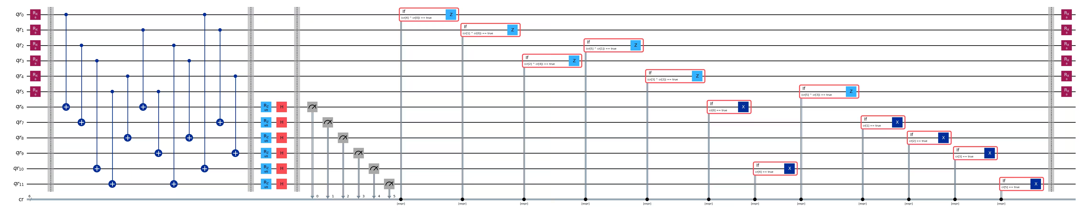
Ang resultang circuit ay ang sumusunod:

Kapag ginamit natin ang pamamaraang ito upang i-simulate ang isang honeycomb lattice, ang resultang circuit ay perpektong naka-embed sa hardware na may heavy-hex lattice: lahat ng data qubit ay nananahan sa mga degree-3 na site ng lattice, na bumubuo ng hexagonal lattice. Bawat pares ng data qubit ay nagbabahagi ng isang ancilla qubit na nananahan sa isang degree-2 na site. Sa ibaba, binubuo natin ang qubit lattice para sa dynamic circuit implementation, na nagpapakilala ng mga ancilla qubit (ipinapakita sa mas maitim na kulay-ube na mga bilog).

def make_lattice(hex_rows=1, hex_cols=1):
    """Define heavy-hex lattice and corresponding lists of data and ancilla nodes."""
    hex_cmap = CouplingMap.from_hexagonal_lattice(
        hex_rows, hex_cols, bidirectional=False
    )
    data = list(hex_cmap.physical_qubits)

    heavyhex_cmap = CouplingMap()
    for d in data:
        heavyhex_cmap.add_physical_qubit(d)

    # make coupling map
    a = len(data)
    for edge in hex_cmap.get_edges():
        heavyhex_cmap.add_physical_qubit(a)
        heavyhex_cmap.add_edge(edge[0], a)
        heavyhex_cmap.add_edge(edge[1], a)
        a += 1
    ancilla = list(range(len(data), a))
    qubits = data + ancilla

    # color edges
    graph = heavyhex_cmap.graph.to_undirected(multigraph=False)
    edge_colors = rx.graph_misra_gries_edge_color(graph)
    layer_edges = {color: [] for color in edge_colors.values()}
    for edge_index, color in edge_colors.items():
        layer_edges[color].append(graph.edge_list()[edge_index])

    # construct observable
    obs_hex = SparsePauliOp.from_sparse_list(
        [("Z", [i], 1 / len(data)) for i in data],
        num_qubits=len(qubits),
    )

    return (data, qubits, ancilla, layer_edges, heavyhex_cmap, graph, obs_hex)

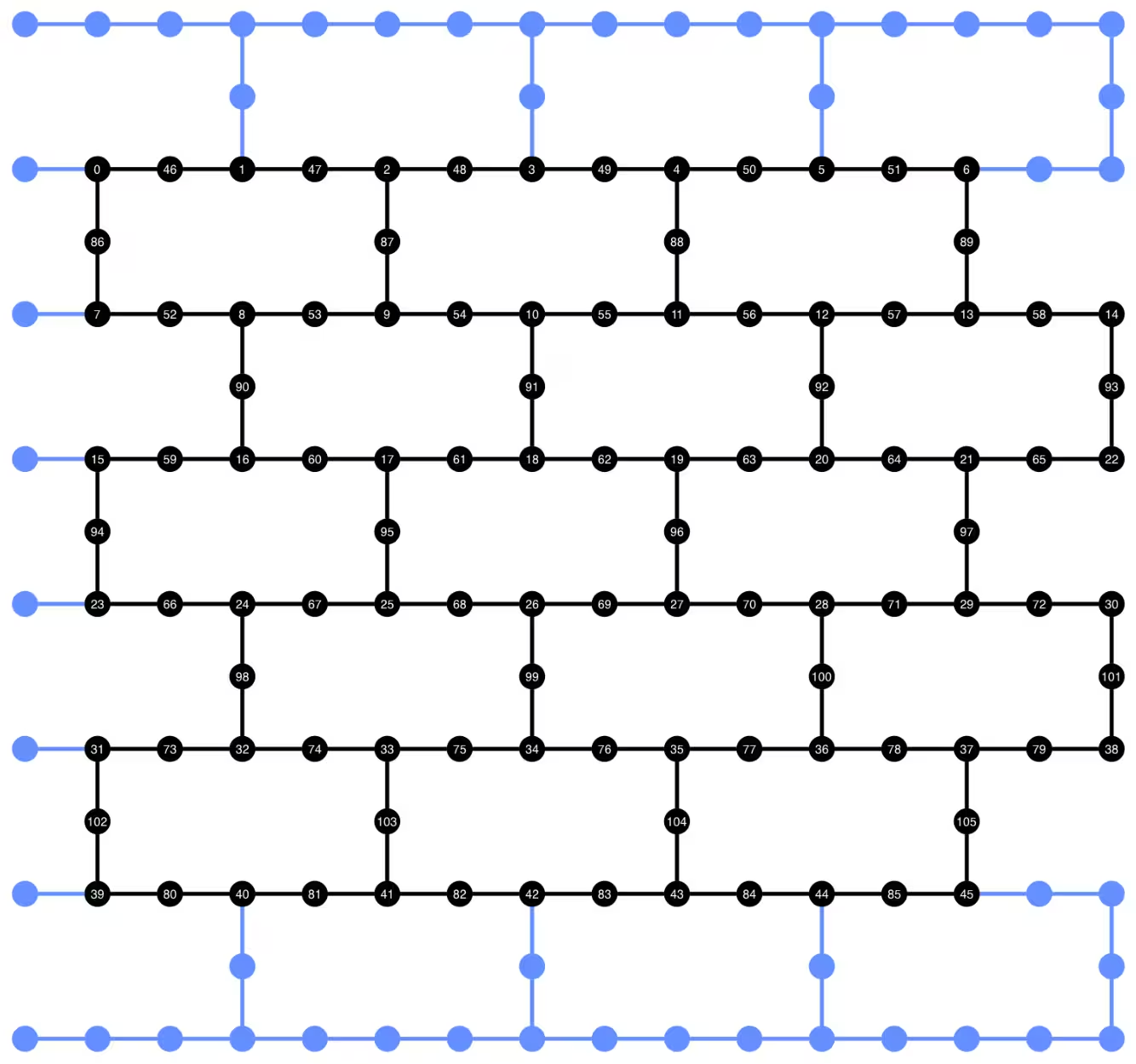
I-visualize ang heavy-hex lattice para sa mga data qubit at ancilla qubit sa maliit na sukat:

(data, qubits, ancilla, layer_edges, heavyhex_cmap, graph, obs_hex) = (
    make_lattice(hex_rows=hex_rows, hex_cols=hex_cols)
)

print(f"number of data qubits = {len(data)}")
print(f"number of ancilla qubits = {len(ancilla)}")

node_colors = []
for node in graph.node_indices():
    if node in ancilla:
        node_colors.append("purple")
    else:
        node_colors.append("lightblue")

pos = rx.graph_spring_layout(
    graph,
    k=1 / np.sqrt(len(qubits)),
    repulsive_exponent=2,
    num_iter=200,
)

# Visualize the graph, blue circles are data qubits and purple circles are ancillas
mpl_draw(graph, node_color=node_colors, pos=pos)
plt.show()

number of data qubits = 46
number of ancilla qubits = 60

Sa ibaba, binubuo natin ang dynamic circuit para sa Trotterized time evolution. Ang mga RZZ gate ay pinapalitan ng dynamic circuit implementation gamit ang mga hakbang na inilarawan sa itaas.

def gen_hex_dynamic(
    depth=1,
    zz_angle=np.pi / 8,
    θ=Parameter("θ"),
    hex_rows=1,
    hex_cols=1,
    measure=False,
    add_dd=True,
):
    """Build dynamic circuits."""
    (data, qubits, ancilla, layer_edges, heavyhex_cmap, graph, obs_hex) = (
        make_lattice(hex_rows=hex_rows, hex_cols=hex_cols)
    )
    # Initialize circuit
    qr = QuantumRegister(len(qubits), "qr")
    cr = ClassicalRegister(len(ancilla), "cr")
    circuit = QuantumCircuit(qr, cr)

    for k in range(depth):
        # Single-qubit Rx layer
        for d in data:
            circuit.rx(θ, d)
        circuit.barrier()

        # CX gates from data qubits to ancilla qubits
        for same_color_edges in layer_edges.values():
            for e in same_color_edges:
                circuit.cx(e[0], e[1])
        circuit.barrier()

        # Apply Rz rotation on ancilla qubits and rotate into X basis
        for a in ancilla:
            circuit.rz(zz_angle, a)
            circuit.h(a)
        # Add barrier to align terminal measurement
        circuit.barrier()

        # Measure ancilla qubits
        for i, a in enumerate(ancilla):
            circuit.measure(a, i)
        d2ros = {}
        a2ro = {}
        # Retrieve ancilla measurement outcomes
        for a in ancilla:
            a2ro[a] = cr[ancilla.index(a)]

        # For each data qubit, retrieve measurement outcomes of neighboring ancilla qubits
        for d in data:
            ros = [a2ro[a] for a in heavyhex_cmap.neighbors(d)]
            d2ros[d] = ros

        # Build classical feedforward operations (optionally add DD on idling data qubits)
        for d in data:
            if add_dd:
                circuit = add_stretch_dd(circuit, d, f"data_{d}_depth_{k}")

            # # XOR the neighboring readouts of the data qubit; if True, apply Z to it
            ros = d2ros[d]
            parity = ros[0]
            for ro in ros[1:]:
                parity = expr.bit_xor(parity, ro)
            with circuit.if_test(expr.equal(parity, True)):
                circuit.z(d)

        # Reset the ancilla if its readout is 1
        for a in ancilla:
            with circuit.if_test(expr.equal(a2ro[a], True)):
                circuit.x(a)
        circuit.barrier()

    # Final single-qubit Rx layer to match the unitary circuits
    for d in data:
        circuit.rx(θ, d)

    if measure:
        circuit.measure_all()
    return circuit, obs_hex

def add_stretch_dd(qc, q, name):
    """Add XpXm DD sequence."""
    s = qc.add_stretch(name)
    qc.delay(s, q)
    qc.x(q)
    qc.delay(s, q)
    qc.delay(s, q)
    qc.rz(np.pi, q)
    qc.x(q)
    qc.rz(-np.pi, q)
    qc.delay(s, q)
    return qc

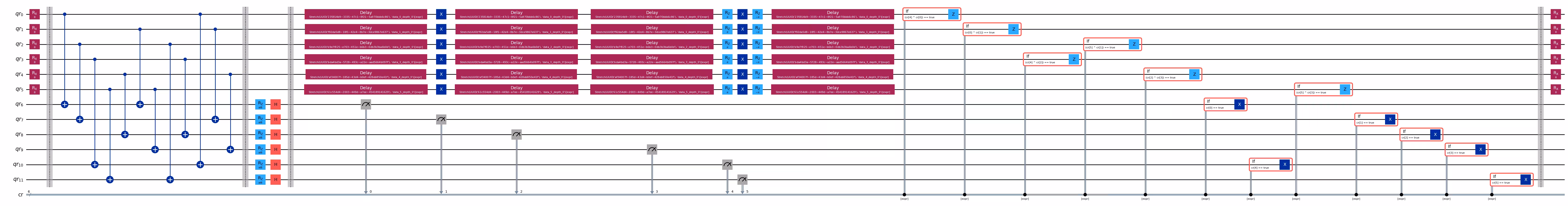
Dynamical decoupling (DD) at suporta para sa stretch duration

Isang caveat ng paggamit ng dynamic circuit implementation upang maisakatuparan ang ZZ interaction ay ang mid-circuit measurement at ang mga klasikal na feedforward operation ay karaniwang mas matagal ipatupad kaysa sa mga quantum gates. Upang mapigilan ang decoherence ng qubit sa panahon ng idle time para sa mga klasikal na operasyon, nagdagdag tayo ng dynamical decoupling (DD) sequence pagkatapos ng operasyon ng pagsukat sa mga ancilla qubit, at bago ang kondisyonal na Z operation sa data qubit, bago ang if_test statement.

Ang DD sequence ay idinadagdag ng function na add_stretch_dd(), na gumagamit ng stretch durations upang matukoy ang mga agwat ng oras sa pagitan ng mga DD gate. Ang stretch duration ay isang paraan upang tukuyin ang isang stretchable na tagal ng oras para sa operasyong delay upang ang tagal ng delay ay maaaring lumaki upang mapuno ang idle time ng qubit. Ang mga duration variable na tinutukoy ng stretch ay nalulutas sa compile time sa mga nais na tagal na nakakatugon sa isang partikular na hadlang. Ito ay napaka-kapaki-pakinabang kapag ang timing ng mga DD sequence ay mahalaga upang makamit ang magandang pagganap ng error suppression. Para sa karagdagang detalye tungkol sa uri ng stretch, tingnan ang dokumentasyon ng OpenQASM. Sa kasalukuyan, ang suporta para sa uri ng stretch sa Qiskit Runtime ay eksperimental pa. Para sa mga detalye tungkol sa mga hadlang sa paggamit nito, pakitingnan ang seksyon ng mga limitasyon ng dokumentasyon ng stretch.

Gamit ang mga function na tinukoy sa itaas, binubuo natin ang mga Trotterized time evolution circuit, na may at walang DD, at ang mga kaugnay na observable. Nagsisimula tayo sa pamamagitan ng pag-visualize ng dynamic circuit ng isang maliit na halimbawa:

hex_rows_test = 1
hex_cols_test = 1

(
    data_test,
    qubits_test,
    ancilla_test,
    layer_edges_test,
    heavyhex_cmap_test,
    graph_test,
    obs_hex_test,
) = make_lattice(hex_rows=hex_rows_test, hex_cols=hex_cols_test)

node_colors = []
for node in graph_test.node_indices():
    if node in ancilla_test:
        node_colors.append("purple")
    else:
        node_colors.append("lightblue")
pos = rx.graph_spring_layout(
    graph_test,
    k=5 / np.sqrt(len(qubits_test)),
    repulsive_exponent=2,
    num_iter=150,
)

# display a small example for illustration
node_colors_test = ["lightblue"] * len(graph_test.node_indices())
mpl_draw(graph_test, node_color=node_colors, pos=pos)

circuit_dynamic_test, obs_dynamic_test = gen_hex_dynamic(
    depth=1,
    θ=Parameter("θ"),
    hex_rows=hex_rows_test,
    hex_cols=hex_cols_test,
    measure=False,
    add_dd=False,
)
circuit_dynamic_test.draw("mpl", fold=-1)

circuit_dynamic_dd_test, _ = gen_hex_dynamic(
    depth=1,
    θ=Parameter("θ"),
    hex_rows=hex_rows_test,
    hex_cols=hex_cols_test,
    measure=False,
    add_dd=True,
)
circuit_dynamic_dd_test.draw("mpl", fold=-1)

Katulad nito, buuin ang mga dynamic circuit para sa malaking halimbawa:

circuits_dynamic = []
circuits_dynamic_dd = []
observables_dynamic = []
for depth in depths:
    circuit, obs = gen_hex_dynamic(
        depth=depth,
        θ=Parameter("θ"),
        hex_rows=hex_rows,
        hex_cols=hex_cols,
        measure=True,
        add_dd=False,
    )
    circuits_dynamic.append(circuit)

    circuit_dd, _ = gen_hex_dynamic(
        depth=depth,
        θ=Parameter("θ"),
        hex_rows=hex_rows,
        hex_cols=hex_cols,
        measure=True,
        add_dd=True,
    )
    circuits_dynamic_dd.append(circuit_dd)
    observables_dynamic.append(obs)

Hakbang 2: I-optimize ang problema para sa pagsasagawa sa hardware

Handa na tayong i-transpile ang circuit sa hardware. I-transpile natin ang parehong unitary standard implementation at ang dynamic circuit implementation sa hardware.

Para ma-transpile sa hardware, kailangan muna nating i-instantiate ang backend. Kung available, pipiliin natin ang backend kung saan sinusuportahan ang MidCircuitMeasure (measure_2) na instruksyon.

service = QiskitRuntimeService()
try:
    backend = service.least_busy(
        operational=True,
        simulator=False,
        use_fractional_gates=True,
        filters=lambda b: "measure_2" in b.supported_instructions,
    )
except QiskitBackendNotFoundError:
    backend = service.least_busy(
        operational=True,
        simulator=False,
        use_fractional_gates=True,
    )

Transpilation para sa mga dynamic circuit

Una, ita-transpile natin ang mga dynamic circuit, na may at walang idinagdag na DD sequence. Upang matiyak na magagamit natin ang parehong hanay ng mga pisikal na qubit sa lahat ng circuit para sa mas magkakaayon na mga resulta, ita-transpile muna natin ang circuit nang isang beses, at pagkatapos ay gagamitin ang layout nito para sa lahat ng kasunod na circuit, na tinukoy ng initial_layout sa pass manager. Pagkatapos ay itatayo natin ang primitive unified blocs (PUBs) bilang input ng Sampler primitive.

pm_temp = generate_preset_pass_manager(
    optimization_level=3,
    backend=backend,
)
isa_temp = pm_temp.run(circuits_dynamic[-1])
dynamic_layout = isa_temp.layout.initial_index_layout(filter_ancillas=True)

pm = generate_preset_pass_manager(
    optimization_level=3, backend=backend, initial_layout=dynamic_layout
)

dynamic_isa_circuits = [pm.run(circ) for circ in circuits_dynamic]
dynamic_pubs = [(circ, params) for circ in dynamic_isa_circuits]

dynamic_isa_circuits_dd = [pm.run(circ) for circ in circuits_dynamic_dd]
dynamic_pubs_dd = [(circ, params) for circ in dynamic_isa_circuits_dd]

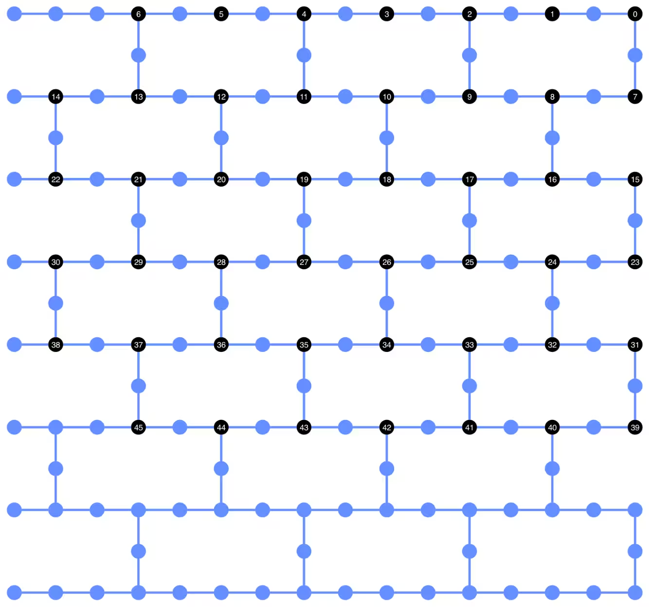
Maaari nating mailarawan ang qubit layout ng transpiled circuit sa ibaba. Ang mga itim na bilog ay nagpapakita ng mga data qubit at ng mga ancilla qubit na ginagamit sa dynamic circuit implementation.

def _heron_coords_r2():
    cord_map = np.array(
        [
            [
                0,
                1,
                2,
                3,
                4,
                5,
                6,
                7,
                8,
                9,
                10,
                11,
                12,
                13,
                14,
                15,
                3,
                7,
                11,
                15,
                0,
                1,
                2,
                3,
                4,
                5,
                6,
                7,
                8,
                9,
                10,
                11,
                12,
                13,
                14,
                15,
                1,
                5,
                9,
                13,
                0,
                1,
                2,
                3,
                4,
                5,
                6,
                7,
                8,
                9,
                10,
                11,
                12,
                13,
                14,
                15,
                3,
                7,
                11,
                15,
                0,
                1,
                2,
                3,
                4,
                5,
                6,
                7,
                8,
                9,
                10,
                11,
                12,
                13,
                14,
                15,
                1,
                5,
                9,
                13,
                0,
                1,
                2,
                3,
                4,
                5,
                6,
                7,
                8,
                9,
                10,
                11,
                12,
                13,
                14,
                15,
                3,
                7,
                11,
                15,
                0,
                1,
                2,
                3,
                4,
                5,
                6,
                7,
                8,
                9,
                10,
                11,
                12,
                13,
                14,
                15,
                1,
                5,
                9,
                13,
                0,
                1,
                2,
                3,
                4,
                5,
                6,
                7,
                8,
                9,
                10,
                11,
                12,
                13,
                14,
                15,
                3,
                7,
                11,
                15,
                0,
                1,
                2,
                3,
                4,
                5,
                6,
                7,
                8,
                9,
                10,
                11,
                12,
                13,
                14,
                15,
            ],
            -1
            * np.array([j for i in range(15) for j in [i] * [16, 4][i % 2]]),
        ],
        dtype=int,
    )

    hcords = []
    ycords = cord_map[0]
    xcords = cord_map[1]
    for i in range(156):
        hcords.append([xcords[i] + 1, np.abs(ycords[i]) + 1])

    return hcords

plot_circuit_layout(
    dynamic_isa_circuits_dd[8],
    backend,
    qubit_coordinates=_heron_coords_r2(),
    view="virtual",
)

tala

Kung makakakuha ka ng mga error tungkol sa neato na hindi nahanap mula sa plot_circuit_layout(), tiyaking naka-install ang graphviz package at available ito sa iyong PATH. Kung nag-i-install ito sa isang hindi default na lokasyon (halimbawa, gamit ang homebrew sa MacOS), maaaring kailanganin mong i-update ang iyong PATH environment variable. Magagawa ito sa loob ng notebook na ito gamit ang sumusunod:

import os
os.environ['PATH'] = f"path/to/neato{os.pathsep}{os.environ['PATH']}"

dynamic_isa_circuits[1].draw(fold=-1, output="mpl", idle_wires=False)

dynamic_isa_circuits_dd[1].draw(fold=-1, output="mpl", idle_wires=False)

Transpile gamit ang MidCircuitMeasure

Ang MidCircuitMeasure ay isang karagdagan sa mga available na operasyon ng pagsukat, na espesyal na kina-calibrate upang magsagawa ng mid-circuit measurements. Ang instruksyong MidCircuitMeasure ay nag-ma-map sa instruksyong measure_2 na sinusuportahan ng mga backend. Tandaan na hindi sinusuportahan ang measure_2 sa lahat ng backend. Maaari mong gamitin ang service.backends(filters=lambda b: "measure_2" in b.supported_instructions) upang mahanap ang mga backend na sumusuporta nito. Dito, ipinapakita natin kung paano i-transpile ang circuit upang ang mga mid-circuit measurement na tinukoy sa circuit ay isasagawa gamit ang operasyong MidCircuitMeasure, kung sinusuportahan ito ng backend.

Sa ibaba, ini-print natin ang tagal para sa instruksyong measure_2 at sa karaniwang instruksyong measure.

print(
    f'Mid-circuit measurement `measure_2` duration: {backend.instruction_durations.get('measure_2',0) * backend.dt * 1e9/1e3} μs'
)
print(
    f'Terminal measurement `measure` duration: {backend.instruction_durations.get('measure',0) * backend.dt *1e9/1e3} μs'
)

Mid-circuit measurement `measure_2` duration:  1.624 μs
Terminal measurement `measure` duration: 2.2 μs

"""Pass that replaces terminal measures in the middle of the circuit with
MidCircuitMeasure instructions."""

class ConvertToMidCircuitMeasure(TransformationPass):
    """This pass replaces terminal measures in the middle of the circuit with
    MidCircuitMeasure instructions.
    """

    def __init__(self, target):
        super().__init__()
        self.target = target

    def run(self, dag):
        """Run the pass on a dag."""
        mid_circ_measure = None
        for inst in self.target.instructions:
            if isinstance(inst[0], Instruction) and inst[0].name.startswith(
                "measure_"
            ):
                mid_circ_measure = inst[0]
                break
        if not mid_circ_measure:
            return dag

        final_measure_nodes = calc_final_ops(dag, {"measure"})
        for node in dag.op_nodes(Measure):
            if node not in final_measure_nodes:
                dag.substitute_node(node, mid_circ_measure, inplace=True)

        return dag

pm = PassManager(ConvertToMidCircuitMeasure(backend.target))

dynamic_isa_circuits_meas2 = [pm.run(circ) for circ in dynamic_isa_circuits]
dynamic_pubs_meas2 = [(circ, params) for circ in dynamic_isa_circuits_meas2]

dynamic_isa_circuits_dd_meas2 = [
    pm.run(circ) for circ in dynamic_isa_circuits_dd
]
dynamic_pubs_dd_meas2 = [
    (circ, params) for circ in dynamic_isa_circuits_dd_meas2
]

Transpilation para sa mga unitary circuit

Upang maitatag ang isang patas na paghahambing sa pagitan ng mga dynamic circuit at ng kanilang katumbas na unitary, ginagamit natin ang parehong hanay ng mga pisikal na qubit na ginagamit sa mga dynamic circuit para sa mga data qubit bilang layout para sa pag-transpile ng mga unitary circuit.

init_layout = [
    dynamic_layout[ind] for ind in range(circuits_unitary[0].num_qubits)
]

pm = generate_preset_pass_manager(
    target=backend.target,
    initial_layout=init_layout,
    optimization_level=3,
)

def transpile_minimize(circ: QuantumCircuit, pm: PassManager, iterations=10):
    """Transpile circuits for specified number of iterations and return the one with smallest two-qubit gate depth"""
    circs = [pm.run(circ) for i in range(iterations)]
    circs_sorted = sorted(
        circs,
        key=lambda x: x.depth(lambda x: x.operation.num_qubits == 2),
    )
    return circs_sorted[0]

unitary_isa_circuits = []
for circ in circuits_unitary:
    circ_t = transpile_minimize(circ, pm, iterations=100)
    unitary_isa_circuits.append(circ_t)

unitary_pubs = [(circ, params) for circ in unitary_isa_circuits]

Inilalarawan natin ang qubit layout ng mga transpiled unitary circuit. Ang mga itim na bilog ay nagpapahiwatig ng mga pisikal na qubit na ginamit upang i-transpile ang mga unitary circuit at ang kanilang mga indeks ay tumutugma sa mga virtual qubit index. Sa pamamagitan ng paghahambing nito sa layout na na-plot para sa mga dynamic circuit, maaari nating kumpirmahin na gumagamit ang mga unitary circuit ng parehong hanay ng mga pisikal na qubit bilang mga data qubit sa mga dynamic circuit.

plot_circuit_layout(
    unitary_isa_circuits[-1],
    backend,
    qubit_coordinates=_heron_coords_r2(),
    view="virtual",
)

Idinaragdag na natin ngayon ang DD sequence sa mga transpiled circuit at itatayo ang mga kaukulang PUB para sa pagsusumite ng trabaho.

pm_dd = PassManager(
    [
        ALAPScheduleAnalysis(target=backend.target),
        PadDynamicalDecoupling(
            dd_sequence=[
                XGate(),
                RZGate(np.pi),
                XGate(),
                RZGate(-np.pi),
            ],
            spacing=[1 / 4, 1 / 2, 0, 0, 1 / 4],
            target=backend.target,
        ),
    ]
)

unitary_isa_circuits_dd = pm_dd.run(unitary_isa_circuits)
unitary_pubs_dd = [(circ, params) for circ in unitary_isa_circuits_dd]

Paghahambing ng two-qubit gate depth ng unitary at dynamic circuit

# compare circuit depth of unitary and dynamic circuit implementations
unitary_depth = [
    unitary_isa_circuits[i].depth(lambda x: x.operation.num_qubits == 2)
    for i in range(len(unitary_isa_circuits))
]

dynamic_depth = [
    dynamic_isa_circuits[i].depth(lambda x: x.operation.num_qubits == 2)
    for i in range(len(dynamic_isa_circuits))
]

plt.plot(
    list(range(len(unitary_depth))),
    unitary_depth,
    label="unitary circuits",
    color="#be95ff",
)
plt.plot(
    list(range(len(dynamic_depth))),
    dynamic_depth,
    label="dynamic circuits",
    color="#ff7eb6",
)
plt.xlabel("Trotter steps")
plt.ylabel("Two-qubit depth")
plt.legend()

<matplotlib.legend.Legend at 0x374225760>

Ang pangunahing benepisyo ng circuit na batay sa pagsukat ay, kapag nagpapatupad ng maraming ZZ interaction, maaaring i-parallelize ang mga CX layer, at maaaring mangyari nang sabay-sabay ang mga pagsukat. Ito ay dahil ang lahat ng ZZ interaction ay nagko-commute, kaya maaaring isagawa ang computation na may measurement depth na 1. Pagkatapos i-transpile ang mga circuit, napansin natin na ang dynamic circuit approach ay nagbubunga ng makabuluhang mas maikling two-qubit depth kaysa sa karaniwang unitary approach, na may caveat na ang mga karagdagang mid-circuit measurement at ang classical feedforward mismo ay tumatagal ng panahon at nagdudulot ng sariling mga pinagmumulan ng mga error.

Hakbang 3: Isagawa gamit ang mga Qiskit primitives

Lokal na mode ng pagsubok

Bago isumite ang mga trabaho sa hardware, maaari tayong magsagawa ng maliit na pagsubok na simulation ng dynamic circuit gamit ang lokal na mode ng pagsubok.

aer_sim = AerSimulator()
pm = generate_preset_pass_manager(backend=aer_sim, optimization_level=1)
circuit_dynamic_test.measure_all()
isa_qc = pm.run(circuit_dynamic_test)
with Batch(backend=aer_sim) as batch:
    sampler = Sampler(mode=batch)
    result = sampler.run([(isa_qc, params)]).result()

print(
    "Simulated average magnetization at trotter step = 1 at three theta values"
)
result[0].data["meas"].expectation_values(obs_dynamic_test[0])

Simulated average magnetization at trotter step = 1 at three theta values

array([ 0.16666667,  0.01855469, -0.13476562])

Simulasyon ng MPS

Para sa malalaking circuit, maaari nating gamitin ang matrix_product_state (MPS) simulator, na nagbibigay ng tinatayang resulta sa halaga ng inaasahang kinalabasan ayon sa napiling bond dimension. Gagamitin natin ang mga resulta ng MPS simulation bilang baseline upang ikumpara ang mga resulta mula sa hardware.

# The MPS simulation below took approximately 7 minutes to run on a laptop with Apple M1 chip

mps_backend = AerSimulator(
    method="matrix_product_state",
    matrix_product_state_truncation_threshold=1e-5,
    matrix_product_state_max_bond_dimension=100,
)
mps_sampler = Aer_Sampler.from_backend(mps_backend)

shots = 4096

data_sim = []
for j in range(points):
    circ_list = [
        circ.assign_parameters([params[j]]) for circ in circuits_unitary
    ]

    mps_job = mps_sampler.run(circ_list, shots=shots)
    result = mps_job.result()

    point_data = [
        result[d].data["meas"].expectation_values(observables_unitary)
        for d in depths
    ]

    data_sim.append(point_data)  # data at one theta value

data_sim = np.array(data_sim)

Sa pagkakahanda ng mga circuit at observable, isasagawa na natin ang mga ito sa hardware gamit ang Sampler primitive.

Dito ay nagsusumite tayo ng tatlong trabaho para sa unitary_pubs, dynamic_pubs, at dynamic_pubs_dd. Ang bawat isa ay isang listahan ng mga parametrized circuit na tumutugma sa siyam na iba't ibang Trotter step na may tatlong iba't ibang parameter na $\theta$.

shots = 10000

with Batch(backend=backend) as batch:
    sampler = Sampler(mode=batch)

    sampler.options.experimental = {
        "execution": {
            "scheduler_timing": True
        },  # set to True to retrieve circuit timing info
    }

    job_unitary = sampler.run(unitary_pubs, shots=shots)
    print(f"unitary: {job_unitary.job_id()}")

    job_unitary_dd = sampler.run(unitary_pubs_dd, shots=shots)
    print(f"unitary_dd: {job_unitary_dd.job_id()}")

    job_dynamic = sampler.run(dynamic_pubs, shots=shots)
    print(f"dynamic: {job_dynamic.job_id()}")

    job_dynamic_dd = sampler.run(dynamic_pubs_dd, shots=shots)
    print(f"dynamic_dd: {job_dynamic_dd.job_id()}")

    job_dynamic_meas2 = sampler.run(dynamic_pubs_meas2, shots=shots)
    print(f"dynamic_meas2: {job_dynamic_meas2.job_id()}")

    job_dynamic_dd_meas2 = sampler.run(dynamic_pubs_dd_meas2, shots=shots)
    print(f"dynamic_dd_meas2: {job_dynamic_dd_meas2.job_id()}")

unitary: d5dtt0ldq8ts73fvbhj0
unitary: d5dtt11smlfc739onuag
dynamic: d5dtt1hsmlfc739onuc0
dynamic_dd: d5dtt25jngic73avdne0
dynamic_meas2: d5dtt2ldq8ts73fvbhm0
dynamic_dd_meas2: d5dtt2tjngic73avdnf0

Hakbang 4: I-post-process at ibalik ang mga resulta sa nais na klasikal na format

Pagkatapos makumpleto ang mga trabaho, maaari nating kunin ang tagal ng circuit mula sa metadata ng mga resulta ng trabaho at i-visualize ang impormasyon ng iskedyul ng circuit. Para sa karagdagang impormasyon tungkol sa pag-visualize ng impormasyon ng pag-iskedyul ng isang circuit, sumangguni po sa pahinang ito.

# Circuit durations is reported in the unit of `dt` which can be retrieved from `Backend` object
unitary_durations = [
    job_unitary.result()[i].metadata["compilation"]["scheduler_timing"][
        "circuit_duration"
    ]
    for i in depths
]

dynamic_durations = [
    job_dynamic.result()[i].metadata["compilation"]["scheduler_timing"][
        "circuit_duration"
    ]
    for i in depths
]

dynamic_durations_meas2 = [
    job_dynamic_meas2.result()[i].metadata["compilation"]["scheduler_timing"][
        "circuit_duration"
    ]
    for i in depths
]

result_dd = job_dynamic_dd.result()[1]
circuit_schedule_dd = result_dd.metadata["compilation"]["scheduler_timing"][
    "timing"
]

# to visualize the circuit schedule, one can show the figure below
fig_dd = draw_circuit_schedule_timing(
    circuit_schedule=circuit_schedule_dd,
    included_channels=None,
    filter_readout_channels=False,
    filter_barriers=False,
    width=1000,
)

# Save to a file since the figure is large
fig_dd.write_html("scheduler_timing_dd.html")

Ini-plot natin ang mga tagal ng circuit para sa mga unitary circuit at sa mga dynamic circuit. Mula sa plot sa ibaba, makikita natin na, kahit may kinakailangang oras para sa mga mid-circuit measurement at klasikal na operasyon, ang pagpapatupad ng dynamic circuit gamit ang measure_2 ay nagbubunga ng katulad na tagal ng circuit kumpara sa pagpapatupad na unitary.

# visualize circuit durations

def convert_dt_to_microseconds(circ_duration: List, backend_dt: float):
    dt = backend_dt * 1e6  # dt in microseconds
    return list(map(lambda x: x * dt, circ_duration))

dt = backend.target.dt
plt.plot(
    depths,
    convert_dt_to_microseconds(unitary_durations, dt),
    color="#be95ff",
    linestyle=":",
    label="unitary",
)
plt.plot(
    depths,
    convert_dt_to_microseconds(dynamic_durations, dt),
    color="#ff7eb6",
    linestyle="-.",
    label="dynamic",
)
plt.plot(
    depths,
    convert_dt_to_microseconds(dynamic_durations_meas2, dt),
    color="#ff7eb6",
    linestyle="-.",
    marker="s",
    mfc="none",
    label="dynamic w/ meas2",
)

plt.xlabel("Trotter steps")
plt.ylabel(r"Circuit durations in $\mu$s")
plt.legend()

<matplotlib.legend.Legend at 0x17f73c6e0>

Pagkatapos makumpleto ang mga trabaho, kinukuha natin ang data sa ibaba at kinakalkula ang average na magnetization na tinatantya ng mga observable na observables_unitary o observables_dynamic na itinayo natin nang mas maaga.

runs = {
    "unitary": (
        job_unitary,
        [observables_unitary] * len(circuits_unitary),
    ),
    "unitary_dd": (
        job_unitary_dd,
        [observables_unitary] * len(circuits_unitary),
    ),
    # Omitting Dyn w/o DD and Dynamic w/ DD plots for better readability
    # "dynamic": (job_dynamic, observables_dynamic),
    # "dynamic_dd": (job_dynamic_dd, observables_dynamic),
    "dynamic_meas2": (job_dynamic_meas2, observables_dynamic),
    "dynamic_dd_meas2": (
        job_dynamic_dd_meas2,
        observables_dynamic,
    ),
}

data_dict = {}
for key, (job, obs) in runs.items():
    data = []
    for i in range(points):
        data.append(
            [
                job.result()[ind].data["meas"].expectation_values(obs[ind])[i]
                for ind in depths
            ]
        )
    data_dict[key] = data

Sa ibaba ay ini-plot natin ang spin magnetization bilang function ng mga Trotter step sa iba't ibang halaga ng $\theta$, na tumutugma sa iba't ibang lakas ng lokal na magnetic field. Ini-plot natin ang parehong pre-computed na mga resulta ng MPS simulation para sa mga ideal na unitary circuit, kasama ang mga eksperimental na resulta mula sa mga sumusunod:

1. pagpapatakbo ng mga unitary circuit na may DD
2. pagpapatakbo ng mga dynamic circuit na may DD at MidCircuitMeasure

plt.figure(figsize=(10, 6))

colors = ["#0f62fe", "#be95ff", "#ff7eb6"]
for i in range(points):
    plt.plot(
        depths,
        data_sim[i],
        color=colors[i],
        linestyle="solid",
        label=f"θ={pi_check(i*max_angle/(points-1))} (MPS)",
    )
    # plt.plot(
    #     depths,
    #     data_dict["unitary"][i],
    #     color=colors[i],
    #     linestyle=":",
    #     label=f"θ={pi_check(i*max_angle/(points-1))} (Unitary)",
    # )

    plt.plot(
        depths,
        data_dict["unitary_dd"][i],
        color=colors[i],
        marker="o",
        mfc="none",
        linestyle=":",
        label=f"θ={pi_check(i*max_angle/(points-1))} (Unitary w/DD)",
    )

    # Omitting Dyn w/o DD and Dynamic w/ DD plots for better readability
    # plt.plot(
    #     depths,
    #     data_dict["dynamic"][i],
    #     color=colors[i],
    #     linestyle="-.",
    #     label=f"θ={pi_check(i*max_angle/(points-1))} (Dyn w/o DD)",
    # )
    # plt.plot(
    #     depths,
    #     data_dict["dynamic_dd"][i],
    #     marker="D",
    #     mfc="none",
    #     color=colors[i],
    #     linestyle="-.",
    #     label=f"θ={pi_check(i*max_angle/(points-1))} (Dynamic w/ DD)",
    # )

    # plt.plot(
    #     depths,
    #     data_dict["dynamic_meas2"][i],
    #     color=colors[i],
    #     marker="s",
    #     mfc="none",
    #     linestyle=':',
    #     label=f"θ={pi_check(i*max_angle/(points-1))} (Dynamic w/ MidCircuitMeas)",
    # )

    plt.plot(
        depths,
        data_dict["dynamic_dd_meas2"][i],
        color=colors[i],
        marker="*",
        markersize=8,
        linestyle=":",
        label=f"θ={pi_check(i*max_angle/(points-1))} (Dynamic w/ DD & MidCircuitMeas)",
    )

plt.xlabel("Trotter steps", fontsize=16)
plt.ylabel("Average magnetization", fontsize=16)
plt.xticks(rotation=45)
handles, labels = plt.gca().get_legend_handles_labels()
plt.legend(
    handles,
    labels,
    loc="upper right",
    bbox_to_anchor=(1.46, 1.0),
    shadow=True,
    ncol=1,
)
plt.title(
    f"{hex_rows}x{hex_cols} hex ring, {num_qubits} data qubits, {len(ancilla)} ancilla qubits \n{backend.name}: Sampler"
)
plt.show()

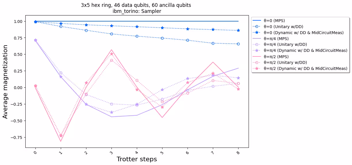
Kapag inihambing natin ang mga eksperimental na resulta sa simulation, makikita nating ang pagpapatupad ng dynamic circuit (tuldok-tuldok na linya na may mga bituin) sa kabuuan ay may mas magandang pagganap kaysa sa karaniwang pagpapatupad na unitary (tuldok-tuldok na linya na may mga bilog). Sa kabuuan, ipinepresenta natin ang mga dynamic circuit bilang solusyon para sa pag-simulate ng mga Ising spin model sa isang honeycomb lattice, isang topology na hindi likas sa hardware. Ang solusyong dynamic circuit ay nagbibigay-daan sa mga ZZ interaction sa pagitan ng mga qubit na hindi pinakamalapit na kapitbahay, na may mas maikling two-qubit gate depth kaysa sa paggamit ng mga SWAP gate, sa halaga ng pagpapakilala ng dagdag na mga ancilla qubit at mga klasikal na feedforward na operasyon.

References

[1] Quantum computing with Qiskit, by Javadi-Abhari, A., Treinish, M., Krsulich, K., Wood, C.J., Lishman, J., Gacon, J., Martiel, S., Nation, P.D., Bishop, L.S., Cross, A.W. and Johnson, B.R., 2024. arXiv preprint arXiv:2405.08810 (2024)