Transverse-Field Ising Model na may Q-CTRL's Performance Management

Pagtatantya ng paggamit: 2 minuto sa Heron r2 processor. (TANDAAN: Ito ay pagtatantya lamang. Ang iyong runtime ay maaaring mag-iba.)

Background

Ang Transverse-Field Ising Model (TFIM) ay mahalaga sa pag-aaral ng quantum magnetism at phase transitions. Inilalarawan nito ang isang set ng spins na nakaayos sa isang lattice, kung saan ang bawat spin ay nakikipag-ugnayan sa mga kapitbahay nito habang naiimpluwensyahan din ng isang external magnetic field na nagdudulot ng quantum fluctuations.

Ang karaniwang diskarte sa pagsisimula ng modelong ito ay ang paggamit ng Trotter decomposition upang tantiyahin ang time evolution operator, na bumubuo ng mga circuits na nagsasalitan sa pagitan ng single-qubit rotations at entangling two-qubit interactions. Gayunpaman, ang simulasyong ito sa tunay na hardware ay mahirap dahil sa ingay at decoherence, na humahantong sa mga paglihis mula sa tunay na dynamics. Upang malampasan ito, ginagamit natin ang Q-CTRL's Fire Opal error suppression at performance management tools, na inaalok bilang isang Qiskit Function (tingnan ang Fire Opal documentation). Awtomatikong ino-optimize ng Fire Opal ang circuit execution sa pamamagitan ng paglalapat ng dynamical decoupling, advanced layout, routing, at iba pang error suppression techniques, na lahat ay naglalayong bawasan ang ingay. Sa mga pagpapahusay na ito, ang mga resulta ng hardware ay mas malapitan sa noiseless simulations, at sa gayon ay maari nating pag-aralan ang TFIM magnetization dynamics na may mas mataas na fidelity.

Sa tutorial na ito ay gagawin natin ang:

• Bumuo ng TFIM Hamiltonian sa isang graph ng mga nakakonektang spin triangles
• Magsimula ng time evolution na may Trotterized circuits sa iba't ibang depths
• Kalkulahin at i-visualize ang single-qubit magnetizations $\langle Z_i \rangle$ sa paglipas ng panahon
• Ihambing ang baseline simulations sa mga resulta mula sa hardware runs gamit ang Q-CTRL's Fire Opal performance management

Overview

Ang Transverse-field Ising Model (TFIM) ay isang quantum spin model na sumasaklaw sa mahahalagang features ng quantum phase transitions. Ang Hamiltonian ay tinukoy bilang:

$$H = -J \sum_{i} Z_i Z_{i+1} - h \sum_{i} X_i$$

kung saan ang $Z_i$ at $X_i$ ay Pauli operators na kumikilos sa qubit $i$, ang $J$ ay ang coupling strength sa pagitan ng magkatabing spins, at ang $h$ ay ang lakas ng transverse magnetic field. Ang unang term ay kumakatawan sa classical ferromagnetic interactions, habang ang pangalawa ay nagpapasok ng quantum fluctuations sa pamamagitan ng transverse field. Upang magsimula ng TFIM dynamics, ginagamit mo ang Trotter decomposition ng unitary evolution operator $e^{-iHt}$, na ipinatupad sa pamamagitan ng mga layer ng RX at RZZ gates batay sa custom graph ng mga nakakonektang spin triangles. Ang simulation ay tumutuklas kung paano umuusad ang magnetization $\langle Z \rangle$ habang tumataas ang Trotter steps.

Ang performance ng iminungkahing TFIM implementation ay tinasa sa pamamagitan ng paghahambing ng noiseless simulations sa noisy backends. Ang Fire Opal's enhanced execution at error suppression features ay ginagamit upang bawasan ang epekto ng ingay sa tunay na hardware, na nagbubunga ng mas maaasahang pagtatantya ng spin observables tulad ng $\langle Z_i \rangle$ at correlators $\langle Z_i Z_j \rangle$.

Requirements

Bago magsimula sa tutorial na ito, tiyaking mayroon kang mga sumusunod na naka-install:

• Qiskit SDK v1.4 o mas bago, na may visualization support
• Qiskit Runtime v0.40 o mas bago (pip install qiskit-ibm-runtime)
• Qiskit Functions Catalog v0.9.0 (pip install qiskit-ibm-catalog)
• Fire Opal SDK v9.0.2 o mas bago (pip install fire-opal)
• Q-CTRL Visualizer v8.0.2 o mas bago (pip install qctrl-visualizer)

Setup

Una, mag-authenticate gamit ang iyong IBM Quantum API key. Pagkatapos, piliin ang Qiskit Function tulad ng sumusunod. (Ang code na ito ay umaasa na na-save mo na ang iyong account sa iyong local environment.)

# Added by doQumentation — required packages for this notebook
!pip install -q matplotlib networkx numpy qctrlvisualizer qiskit qiskit-aer qiskit-ibm-catalog qiskit-ibm-runtime

from qiskit.transpiler.preset_passmanagers import generate_preset_pass_manager
from qiskit import QuantumCircuit
from qiskit_ibm_catalog import QiskitFunctionsCatalog
from qiskit_ibm_runtime import QiskitRuntimeService
from qiskit_ibm_runtime import SamplerV2 as Sampler
from qiskit.quantum_info import SparsePauliOp
from qiskit_aer import AerSimulator

import numpy as np
import networkx as nx
import matplotlib.pyplot as plt
import qctrlvisualizer as qv

catalog = QiskitFunctionsCatalog(channel="ibm_quantum_platform")

# Access Function
perf_mgmt = catalog.load("q-ctrl/performance-management")

Step 1: Map classical inputs to a quantum problem

Generate TFIM graph

Magsisimula tayo sa pamamagitan ng pagtukoy sa lattice ng spins at ng mga couplings sa pagitan nila. Sa tutorial na ito, ang lattice ay itinayo mula sa mga nakakonektang triangles na nakaayos sa isang linear chain. Ang bawat triangle ay binubuo ng tatlong nodes na nakakonekta sa isang saradong loop, at ang chain ay nabuo sa pamamagitan ng pag-uugnay ng isang node ng bawat triangle sa nakaraang triangle.

Ang helper function na connected_triangles_adj_matrix ay bumubuo ng adjacency matrix para sa istrukturang ito. Para sa isang chain ng $n$ triangles, ang resultang graph ay naglalaman ng $2n+1$ nodes.

def connected_triangles_adj_matrix(n):
    """
    Generate the adjacency matrix for 'n' connected triangles in a chain.
    """
    num_nodes = 2 * n + 1
    adj_matrix = np.zeros((num_nodes, num_nodes), dtype=int)

    for i in range(n):
        a, b, c = i * 2, i * 2 + 1, i * 2 + 2  # Nodes of the current triangle

        # Connect the three nodes in a triangle
        adj_matrix[a, b] = adj_matrix[b, a] = 1
        adj_matrix[b, c] = adj_matrix[c, b] = 1
        adj_matrix[a, c] = adj_matrix[c, a] = 1

        # If not the first triangle, connect to the previous triangle
        if i > 0:
            adj_matrix[a, a - 1] = adj_matrix[a - 1, a] = 1

    return adj_matrix

Upang i-visualize ang lattice na katatapos lang nating tukuyin, maaari nating i-plot ang chain ng mga nakakonektang triangles at lagyan ng label ang bawat node. Ang function sa ibaba ay bumubuo ng graph para sa napiling bilang ng triangles at ipinapakita ito.

def plot_triangle_chain(n, side=1.0):
    """
    Plot a horizontal chain of n equilateral triangles.
    Baseline: even nodes (0,2,4,...,2n) on y=0
    Apexes: odd nodes (1,3,5,...,2n-1) above the midpoint.
    """
    # Build graph
    A = connected_triangles_adj_matrix(n)
    G = nx.from_numpy_array(A)

    h = np.sqrt(3) / 2 * side
    pos = {}

    # Place baseline nodes
    for k in range(n + 1):
        pos[2 * k] = (k * side, 0.0)

    # Place apex nodes
    for k in range(n):
        x_left = pos[2 * k][0]
        x_right = pos[2 * k + 2][0]
        pos[2 * k + 1] = ((x_left + x_right) / 2, h)

    # Draw
    fig, ax = plt.subplots(figsize=(1.5 * n, 2.5))
    nx.draw(
        G,
        pos,
        ax=ax,
        with_labels=True,
        font_size=10,
        font_color="white",
        node_size=600,
        node_color=qv.QCTRL_STYLE_COLORS[0],
        edge_color="black",
        width=2,
    )
    ax.set_aspect("equal")
    ax.margins(0.2)
    plt.show()

    return G, pos

Para sa tutorial na ito ay gagamitin natin ang isang chain ng 20 triangles.

n_triangles = 20
n_qubits = 2 * n_triangles + 1
plot_triangle_chain(n_triangles, side=1.0)
plt.show()

Coloring graph edges

Upang ipatupad ang spin–spin coupling, kapaki-pakinabang na pagsama-samahin ang mga edges na hindi magkakapatong. Pinapayagan tayo nitong maglapat ng two-qubit gates nang sabay-sabay. Magagawa natin ito gamit ang isang simpleng edge-coloring procedure [1], na nag-aatas ng kulay sa bawat edge upang ang mga edges na nagkikita sa parehong node ay mailagay sa magkaibang mga grupo.

def edge_coloring(graph):
    """
    Takes a NetworkX graph and returns a list of lists where each inner list contains
    the edges assigned the same color.
    """
    line_graph = nx.line_graph(graph)
    edge_colors = nx.coloring.greedy_color(line_graph)

    color_groups = {}
    for edge, color in edge_colors.items():
        if color not in color_groups:
            color_groups[color] = []
        color_groups[color].append(edge)

    return list(color_groups.values())

Step 2: Optimize problem for quantum hardware execution

Generate Trotterized circuits on spin graphs

Upang magsimula ng dynamics ng TFIM, bubuo tayo ng mga circuits na tumantiya sa time evolution operator.

$$U(t) = e^{-i H t}, \quad \text{where} \quad H = -J \sum_{\langle i,j \rangle} Z_i Z_j - h \sum_i X_i .$$

Ginagamit natin ang second-order Trotter decomposition:

$$e^{-i H \Delta t} \approx e^{-i H_X \Delta t / 2}\, e^{-i H_Z \Delta t}\, e^{-i H_X \Delta t / 2},$$

kung saan ang $H_X = -h \sum_i X_i$ at ang $H_Z = -J \sum_{\langle i,j \rangle} Z_i Z_j$.

• Ang $H_X$ term ay ipinatupad gamit ang mga layer ng RX rotations.
• Ang $H_Z$ term ay ipinatupad gamit ang mga layer ng RZZ gates kasama ng mga edges ng interaction graph.

Ang mga angles ng gates na ito ay tinutukoy ng transverse field $h$, ng coupling constant $J$, at ng time step $\Delta t$. Sa pamamagitan ng pag-stack ng maraming Trotter steps, bumubuo tayo ng mga circuits na may tumataas na depth na tumantiya sa dynamics ng system. Ang mga functions na generate_tfim_circ_custom_graph at trotter_circuits ay bumubuo ng Trotterized quantum circuit mula sa arbitrary spin interaction graph.

def generate_tfim_circ_custom_graph(
    steps, h, J, dt, psi0, graph: nx.graph.Graph, meas_basis="Z", mirror=False
):
    """
    Generate a second order trotter of the form e^(a+b) ~ e^(b/2) e^a e^(b/2) for simulating a transverse field ising model:
    e^{-i H t} where the Hamiltonian H = -J \\sum_i Z_i Z_{i+1} + h \\sum_i X_i.

    steps: Number of trotter steps
    theta_x: Angle for layer of X rotations
    theta_zz: Angle for layer of ZZ rotations
    theta_x: Angle for second layer of X rotations
    J: Coupling between nearest neighbor spins
    h: The transverse magnetic field strength
    dt: t/total_steps
    psi0: initial state (assumed to be prepared in the computational basis).
    meas_basis: basis to measure all correlators in

    This is a second order trotter of the form e^(a+b) ~ e^(b/2) e^a e^(b/2)
    """
    theta_x = h * dt
    theta_zz = -2 * J * dt
    nq = graph.number_of_nodes()
    color_edges = edge_coloring(graph)
    circ = QuantumCircuit(nq, nq)
    # Initial state, for typical cases in the computational basis
    for i, b in enumerate(psi0):
        if b == "1":
            circ.x(i)
    # Trotter steps
    for step in range(steps):
        for i in range(nq):
            circ.rx(theta_x, i)
        if mirror:
            color_edges = [sublist[::-1] for sublist in color_edges[::-1]]
        for edge_list in color_edges:
            for edge in edge_list:
                circ.rzz(theta_zz, edge[0], edge[1])
        for i in range(nq):
            circ.rx(theta_x, i)

    # some typically used basis rotations
    if meas_basis == "X":
        for b in range(nq):
            circ.h(b)
    elif meas_basis == "Y":
        for b in range(nq):
            circ.sdg(b)
            circ.h(b)

    for i in range(nq):
        circ.measure(i, i)

    return circ

def trotter_circuits(G, d_ind_tot, J, h, dt, meas_basis, mirror=True):
    """
    Generates a sequence of Trotterized circuits, each with increasing depth.
    Given a spin interaction graph and Hamiltonian parameters, it constructs
    a list of circuits with 1 to d_ind_tot Trotter steps

    G: Graph defining spin interactions (edges = ZZ couplings)
    d_ind_tot: Number of Trotter steps (maximum depth)
    J: Coupling between nearest neighboring spins
    h: Transverse magnetic field strength
    dt: (t / total_steps
    meas_basis: Basis to measure all correlators in
    mirror: If True, mirror the Trotter layers
    """
    qubit_count = len(G)
    circuits = []
    psi0 = "0" * qubit_count

    for steps in range(1, d_ind_tot + 1):
        circuits.append(
            generate_tfim_circ_custom_graph(
                steps, h, J, dt, psi0, G, meas_basis, mirror
            )
        )
    return circuits

Estimate single-qubit magnetizations $\langle Z_i \rangle$

Upang pag-aralan ang dynamics ng model, nais nating sukatin ang magnetization ng bawat qubit, na tinukoy ng expectation value $\langle Z_i \rangle = \langle \psi | Z_i | \psi \rangle$.

Sa mga simulations, maari nating kalkulahin ito nang direkta mula sa measurement outcomes. Ang function na z_expectation ay pumoproseso ng bitstring counts at ibinabalik ang value ng $\langle Z_i \rangle$ para sa napiling qubit index. Sa tunay na hardware, sinusuri natin ang parehong quantity sa pamamagitan ng pagtukoy ng Pauli operator gamit ang function na generate_z_observables, at pagkatapos ay kinakalkula ng backend ang expectation value.

def z_expectation(counts, index):
    """
    counts: Dict of mitigated bitstrings.
    index: Index i in the single operator expectation value < II...Z_i...I > to be calculated.
    return:  < Z_i >
    """
    z_exp = 0
    tot = 0
    for bitstring, value in counts.items():
        bit = int(bitstring[index])
        sign = 1
        if bit % 2 == 1:
            sign = -1
        z_exp += sign * value
        tot += value

    return z_exp / tot

def generate_z_observables(nq):
    observables = []
    for i in range(nq):
        pauli_string = "".join(["Z" if j == i else "I" for j in range(nq)])
        observables.append(SparsePauliOp(pauli_string))
    return observables

observables = generate_z_observables(n_qubits)

Tutukuyin na natin ngayon ang mga parameters para sa pagbuo ng Trotterized circuits. Sa tutorial na ito, ang lattice ay isang chain ng 20 nakakonektang triangles, na tumutugma sa isang 41-qubit system.

all_circs_mirror = []
for num_triangles in [n_triangles]:
    for meas_basis in ["Z"]:
        A = connected_triangles_adj_matrix(num_triangles)
        G = nx.from_numpy_array(A)
        nq = len(G)
        d_ind_tot = 22
        dt = 2 * np.pi * 1 / 30 * 0.25
        J = 1
        h = -7
        all_circs_mirror.extend(
            trotter_circuits(G, d_ind_tot, J, h, dt, meas_basis, True)
        )
circs = all_circs_mirror

Step 3: Execute using Qiskit primitives

Run MPS simulation

Ang listahan ng Trotterized circuits ay isinagawa gamit ang matrix_product_state simulator na may arbitrary na pagpili ng $4096$ shots. Ang MPS method ay nagbibigay ng efficient approximation ng circuit dynamics, na may accuracy na tinutukoy ng napiling bond dimension. Para sa mga laki ng system na isinasaalang-alang dito, ang default bond dimension ay sapat na upang makuha ang magnetization dynamics na may mataas na fidelity. Ang raw counts ay na-normalize, at mula dito ay kinakalkula natin ang single-qubit expectation values $\langle Z_i \rangle$ sa bawat Trotter step. Sa wakas, kinakalkula natin ang average sa lahat ng qubits upang makakuha ng isang curve na nagpapakita kung paano nagbabago ang magnetization sa paglipas ng panahon.

backend_sim = AerSimulator(method="matrix_product_state")

def normalize_counts(counts_list, shots):
    new_counts_list = []
    for counts in counts_list:
        a = {k: v / shots for k, v in counts.items()}
        new_counts_list.append(a)
    return new_counts_list

def run_sim(circ_list):
    shots = 4096
    res = backend_sim.run(circ_list, shots=shots)
    normed = normalize_counts(res.result().get_counts(), shots)
    return normed

sim_counts = run_sim(circs)

Run on hardware

service = QiskitRuntimeService()
backend = service.backend("ibm_marrakesh")

def run_qiskit(circ_list):
    shots = 4096
    pm = generate_preset_pass_manager(backend=backend)
    isa_circuits = [pm.run(qc) for qc in circ_list]
    sampler = Sampler(mode=backend)
    res = sampler.run(isa_circuits, shots=shots)
    res = [r.data.c.get_counts() for r in res.result()]
    normed = normalize_counts(res, shots)
    return normed

qiskit_counts = run_qiskit(circs)

Run on hardware with Fire Opal

Sinusuri natin ang magnetization dynamics sa tunay na quantum hardware. Ang Fire Opal ay nagbibigay ng isang Qiskit Function na pinalalawig ang karaniwang Qiskit Runtime Estimator primitive na may automated error suppression at performance management. Isinusubmit natin ang Trotterized circuits nang direkta sa isang IBM® backend habang hinahawakan ng Fire Opal ang noise-aware execution.

Naghahanda tayo ng isang listahan ng pubs, kung saan ang bawat item ay naglalaman ng circuit at ng kaukulang Pauli-Z observables. Ang mga ito ay ipinasa sa estimator function ng Fire Opal, na nagbabalik ng expectation values $\langle Z_i \rangle$ para sa bawat qubit sa bawat Trotter step. Ang mga resulta ay maaaring i-average sa mga qubits upang makuha ang magnetization curve mula sa hardware.

backend_name = "ibm_marrakesh"
estimator_pubs = [(qc, observables) for qc in all_circs_mirror[:]]

# Run the circuit using the estimator
qctrl_estimator_job = perf_mgmt.run(
    primitive="estimator",
    pubs=estimator_pubs,
    backend_name=backend_name,
    options={"default_shots": 4096},
)

result_qctrl = qctrl_estimator_job.result()

Step 4: Post-process and return result in desired classical format

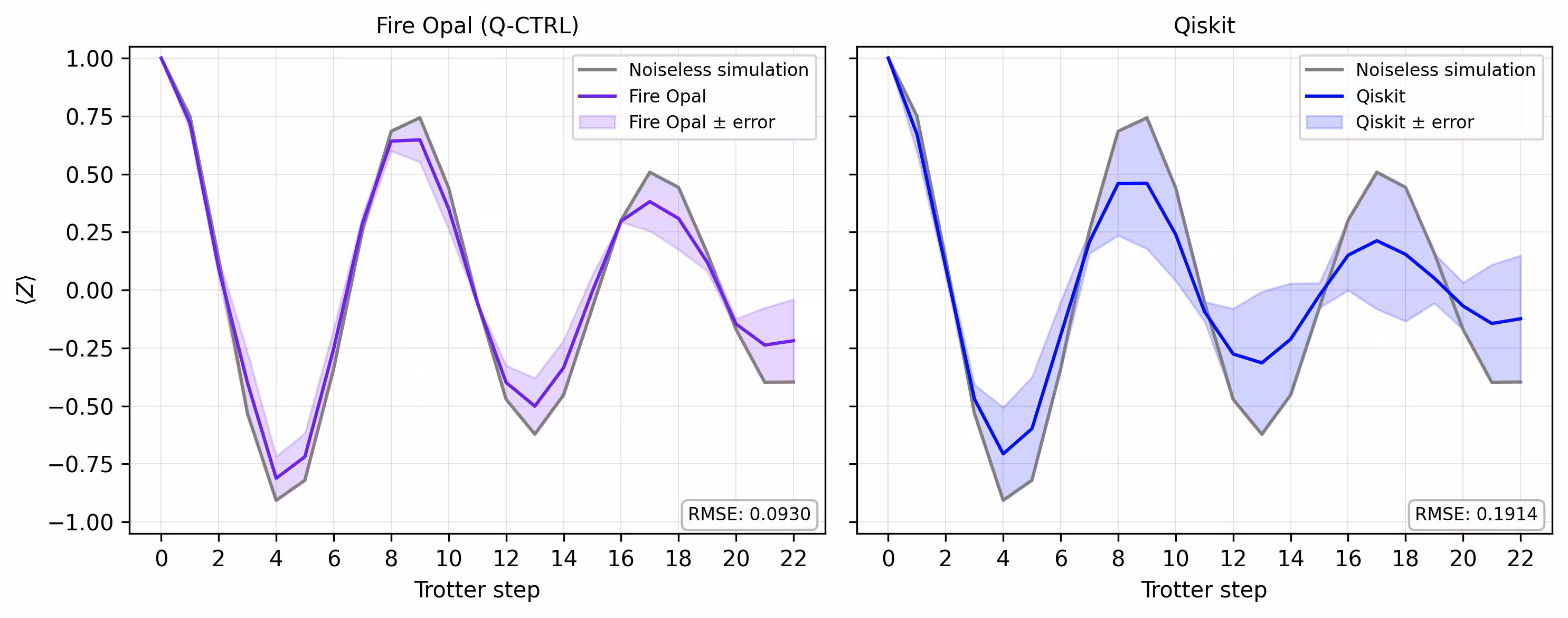
Sa wakas, inihahambing natin ang magnetization curve mula sa simulator sa mga resultang nakuha sa tunay na hardware. Ang pag-plot ng pareho side by side ay nagpapakita kung gaano kalapit ang tugma ng hardware execution na may Fire Opal sa noiseless baseline sa buong Trotter steps.

def make_correlators(test_counts, nq, d_ind_tot):
    mz = np.empty((nq, d_ind_tot))
    for d_ind in range(d_ind_tot):
        counts = test_counts[d_ind]
        for i in range(nq):
            mz[i, d_ind] = z_expectation(counts, i)
    average_z = np.mean(mz, axis=0)
    return np.concatenate((np.array([1]), average_z), axis=0)

sim_exp = make_correlators(sim_counts[0:22], nq=nq, d_ind_tot=22)
qiskit_exp = make_correlators(qiskit_counts[0:22], nq=nq, d_ind_tot=22)

qctrl_exp = [ev.data.evs for ev in result_qctrl[:]]
qctrl_exp_mean = np.concatenate(
    (np.array([1]), np.mean(qctrl_exp, axis=1)), axis=0
)

def make_expectations_plot(
    sim_z,
    depths,
    exp_qctrl=None,
    exp_qctrl_error=None,
    exp_qiskit=None,
    exp_qiskit_error=None,
    plot_from=0,
    plot_upto=23,
):
    import numpy as np
    import matplotlib.pyplot as plt

    depth_ticks = [0, 2, 4, 6, 8, 10, 12, 14, 16, 18, 20, 22]

    d = np.asarray(depths)[plot_from:plot_upto]
    sim = np.asarray(sim_z)[plot_from:plot_upto]

    qk = (
        None
        if exp_qiskit is None
        else np.asarray(exp_qiskit)[plot_from:plot_upto]
    )
    qc = (
        None
        if exp_qctrl is None
        else np.asarray(exp_qctrl)[plot_from:plot_upto]
    )

    qk_err = (
        None
        if exp_qiskit_error is None
        else np.asarray(exp_qiskit_error)[plot_from:plot_upto]
    )
    qc_err = (
        None
        if exp_qctrl_error is None
        else np.asarray(exp_qctrl_error)[plot_from:plot_upto]
    )

    # ---- helper(s) ----
    def rmse(a, b):
        if a is None or b is None:
            return None
        a = np.asarray(a, dtype=float)
        b = np.asarray(b, dtype=float)
        mask = np.isfinite(a) & np.isfinite(b)
        if not np.any(mask):
            return None
        diff = a[mask] - b[mask]
        return float(np.sqrt(np.mean(diff**2)))

    def plot_panel(ax, method_y, method_err, color, label, band_color=None):
        # Noiseless reference
        ax.plot(d, sim, color="grey", label="Noiseless simulation")

        # Method line + band
        if method_y is not None:
            ax.plot(d, method_y, color=color, label=label)
            if method_err is not None:
                lo = np.clip(method_y - method_err, -1.05, 1.05)
                hi = np.clip(method_y + method_err, -1.05, 1.05)
                ax.fill_between(
                    d,
                    lo,
                    hi,
                    alpha=0.18,
                    color=band_color if band_color else color,
                    label=f"{label} ± error",
                )
        else:
            ax.text(
                0.5,
                0.5,
                "No data",
                transform=ax.transAxes,
                ha="center",
                va="center",
                fontsize=10,
                color="0.4",
            )

        # RMSE box (vs sim)
        r = rmse(method_y, sim)
        if r is not None:
            ax.text(
                0.98,
                0.02,
                f"RMSE: {r:.4f}",
                transform=ax.transAxes,
                va="bottom",
                ha="right",
                fontsize=8,
                bbox=dict(
                    boxstyle="round,pad=0.35", fc="white", ec="0.7", alpha=0.9
                ),
            )
        # Axes
        ax.set_xticks(depth_ticks)
        ax.set_ylim(-1.05, 1.05)
        ax.grid(True, which="both", linewidth=0.4, alpha=0.4)
        ax.set_axisbelow(True)
        ax.legend(prop={"size": 8}, loc="best")

    fig, axes = plt.subplots(1, 2, figsize=(10, 4), dpi=300, sharey=True)

    axes[0].set_title("Fire Opal (Q-CTRL)", fontsize=10)
    plot_panel(
        axes[0],
        qc,
        qc_err,
        color="#680CE9",
        label="Fire Opal",
        band_color="#680CE9",
    )
    axes[0].set_xlabel("Trotter step")
    axes[0].set_ylabel(r"$\langle Z \rangle$")
    axes[1].set_title("Qiskit", fontsize=10)
    plot_panel(
        axes[1], qk, qk_err, color="blue", label="Qiskit", band_color="blue"
    )
    axes[1].set_xlabel("Trotter step")

    plt.tight_layout()
    plt.show()

depths = list(range(d_ind_tot + 1))
errors = np.abs(np.array(qctrl_exp_mean) - np.array(sim_exp))

errors_qiskit = np.abs(np.array(qiskit_exp) - np.array(sim_exp))

make_expectations_plot(
    sim_exp,
    depths,
    exp_qctrl=qctrl_exp_mean,
    exp_qctrl_error=errors,
    exp_qiskit=qiskit_exp,
    exp_qiskit_error=errors_qiskit,
)

References

[1] Graph coloring. Wikipedia. Retrieved September 15, 2025, from https://en.wikipedia.org/wiki/Graph_coloring

Tutorial survey

Mangyaring maglaan ng isang minuto upang magbigay ng feedback sa tutorial na ito. Ang inyong mga pananaw ay makakatulong sa amin na mapahusay ang aming mga alok sa nilalaman at karanasan ng user.

Link to survey