Warm-start QAOA gamit ang Optimization Mapper Qiskit addon

Usage estimate: 9 minuto sa Heron r3 (TANDAAN: Isa lang itong tantiya. Maaaring iba ang runtime mo.)

Mga Resulta ng Pagkatuto

• Kung paano i-map ang max-cut problem patungo sa quantum Quadratic Unconstrained Binary Optimization (QUBO) formulation gamit ang qiskit-addon-opt-mapper

• Kung paano magpatupad at magpatakbo ng standard QAOA sa simulator

• Kung paano mag-apply ng WS-QAOA sa pamamagitan ng pagkalkula ng quadratic program (QP) relaxation at pagbuo ng warm-start circuit

• Kung paano ihambing ang energy convergence at kalidad ng solusyon sa pagitan ng standard QAOA at WS-QAOA

Prerequisites

• QAOA tutorial

• Advanced QAOA tutorial

Background

Ang Quantum Approximate Optimization Algorithm (QAOA) ay isang hybrid quantum-classical algorithm na idinisenyo para lutasin ang mga combinatorial optimization problem tulad ng max-cut at pangkalahatang QUBO formulations. Para sa pundasyunal na panimula sa QAOA sa Qiskit, tingnan ang QAOA tutorial; para sa mas advanced na circuit-building techniques, tingnan ang advanced QAOA tutorial.

Sa standard QAOA:

• Ang initial state ay ang uniform superposition $|+\rangle^{\otimes n}$.
• Random na na-initialize ang variational parameters.
• Ang classical optimizer ay naghahanap ng mga parameter na nagpapaliit sa cost function.

Gayunpaman, para sa praktikal na laki ng problema at maingay (noisy) na quantum hardware, ang random initialization ay maaaring magresulta sa mabagal na convergence, mahihinang local minima, at pagtaas ng optimization cost.

Pinapabuti ito ng Warm-start QAOA (WS-QAOA) sa pamamagitan ng pagsasama ng mga insight mula sa classical optimization nang direkta sa quantum circuit. Sinusunod ng tutorial na ito ang mga metodo na ipinakilala nina Egger, Mareček, at Woerner sa Warm-starting quantum optimization. Ang pangunahing ideya ay:

1. Lutasin ang continuous relaxation ng orihinal na binary problem (isang quadratic program sa $[0,1]^n$ sa halip na $\{0,1\}^n$).

2. I-encode ang relaxed solution $c^*_i \in [0,1]$ patungo sa custom initial state gamit ang $Y$-rotation angles $\theta_i = 2\arcsin(\sqrt{c^*_i})$, para ang qubit $i$ ay magsisimula sa isang state kung saan ang probability ng pagsukat ng $|1\rangle$ ay $c^*_i$.

3. Palitan ang standard $X$-mixer ng custom mixer na ang ground state ay ang warm-start initial state, tinitiyak na ang algorithm ay nagsisimula malapit sa classical solution at kayang tuklasin ang paligid nito.

Isang regularization parameter na $\varepsilon \in [0, 0.5]$ ay nagki-clip sa $c^*_i$ palayo sa 0 at 1 para maiwasan ang reachability issues; ang mga qubit na na-initialize sa $|0\rangle$ o $|1\rangle$ ay hindi maaaring galawin ng cost Hamiltonian. Sa $\varepsilon = 0.5$, ang WS-QAOA ay eksaktong nababawas patungo sa standard QAOA.

Ginagamit ng problem modeling ang qiskit-addon-opt-mapper package, na ang Maxcut application class ay bumubuo ng QUBO nang direkta mula sa graph, at ang mga converter at translator nito ay nagma-map sa nagresultang problema patungo sa quantum Hamiltonians.

Requirements

Bago simulan ang tutorial na ito, siguraduhing na-install mo na ang mga sumusunod:

• Qiskit SDK v2.0 o mas bago, na may suportang visualization

• Qiskit Runtime v0.43 o mas bago (pip install qiskit-ibm-runtime)

• Optimization Mapper Qiskit addon (pip install qiskit-addon-opt-mapper)

• SciPy (pip install scipy)

• NetworkX (pip install networkx)

Setup

I-import ang lahat ng kinakailangang library at i-define ang mga helper function na gagamitin sa buong tutorial na ito.

# Added by doQumentation — required packages for this notebook
!pip install -q matplotlib networkx numpy qiskit qiskit-addon-opt-mapper qiskit-ibm-runtime scipy

import numpy as np
import matplotlib.pyplot as plt
import networkx as nx
from scipy.optimize import minimize

from qiskit.circuit import QuantumCircuit, ParameterVector
from qiskit.circuit.library import qaoa_ansatz
from qiskit.quantum_info import Statevector
from qiskit.primitives import StatevectorEstimator, StatevectorSampler
from qiskit.transpiler.preset_passmanagers import generate_preset_pass_manager
from qiskit_ibm_runtime import (
    QiskitRuntimeService,
    Session,
    EstimatorOptions,
    EstimatorV2 as Estimator,
    SamplerV2 as Sampler,
)

from qiskit_addon_opt_mapper.applications import Maxcut
from qiskit_addon_opt_mapper.converters import OptimizationProblemToQubo
from qiskit_addon_opt_mapper.translators import to_ising

Small-scale simulator example

Gumagamit kami ng maliit na max-cut na problema sa isang weighted graph bilang aming running example. Itinatanong ng Max-cut: batay sa isang graph $G=(V,E)$ na may edge weights $w_{ij}$, hanapin ang isang partisyon ng mga vertex sa dalawang set na $S$ at $\bar{S}$ na nagpapalaki sa kabuuang bigat ng mga edge na tumatawid sa cut.

Bilang isang QUBO minimization problem, ang max-cut ay maaaring isulat bilang: $\min_{x \in \{0,1\}^n} -\sum_{(i,j) \in E} w_{ij}(x_i + x_j - 2x_i x_j)$

Gumagamit kami ng four-node graph para sa tractability sa isang simulator.

Hakbang 1: I-map ang mga classical input sa isang quantum problem

Dine-define namin ang max-cut problem gamit ang Maxcut application class mula sa qiskit-addon-opt-mapper, na bumubuo ng QUBO formulation nang direkta mula sa graph. Pagkatapos ay kina-convert namin ito sa QUBO at isinasalin sa Ising Hamiltonian (SparsePauliOp) na angkop para sa QAOA. Nireresolba rin namin ang continuous relaxation ng QUBO — pinapalitan ang binary constraint na $x_i \in \{0,1\}$ ng $x_i \in [0,1]$ — para makuha ang warm-start initial point na $c^*$.

# Define a 4-node weighted graph for the max-cut problem
n_nodes = 4
edges = [(0, 1, 1.0), (0, 2, 1.0), (1, 2, 1.0), (1, 3, 1.0), (2, 3, 1.0)]

G = nx.Graph()
G.add_nodes_from(range(n_nodes))
G.add_weighted_edges_from(edges)

pos = nx.spring_layout(G, seed=42)
edge_labels = {(u, v): d["weight"] for u, v, d in G.edges(data=True)}

fig, ax = plt.subplots(figsize=(4, 3))
nx.draw(G, pos, with_labels=True, node_color="lightblue", ax=ax)
nx.draw_networkx_edge_labels(G, pos, edge_labels=edge_labels, ax=ax)
ax.set_title("Max-Cut graph")
plt.tight_layout()
plt.show()

Ang graph ay may limang edge. Ang optimal na max-cut ay naghihiwalay sa mga node patungo sa $S = \{0, 3\}$ at $\bar{S} = \{1, 2\}$ (o ang complement nito), pinuputol ang apat sa limang edge para sa cut value na 4.

# Build the max-cut problem directly from the NetworkX graph using the
# Maxcut application class. Internally it constructs the QUBO
#   minimize  -sum_{(i,j) in E} w_ij * (x_i + x_j - 2*x_i*x_j)
# (each edge contributes -w to the linear terms and +2w to the quadratic
# term), so we get the same OptimizationProblem without the boilerplate.
maxcut = Maxcut(G)
prob = maxcut.to_optimization_problem()
print(prob.prettyprint())

Problem name: Max-cut

Maximize
  -2*x_0*x_1 - 2*x_0*x_2 - 2*x_1*x_2 - 2*x_1*x_3 - 2*x_2*x_3 + 2*x_0 + 3*x_1
  + 3*x_2 + 2*x_3

Subject to
  No constraints

  Binary variables (4)
    x_0 x_1 x_2 x_3

Binabalot ng Maxcut class ang QUBO construction para hindi na namin kailangang i-expand ang max-cut objective nang manu-mano. Ipinapakita ng nakalimbag na objective ang linear coefficient ng bawat variable (kung gaano ito kontribuyente sa cut) at ang quadratic coefficient ng bawat cross-term (ang parusa sa paglalagay ng dalawang katabing node sa parehong panig). Ang pinagbabatayang OptimizationProblem na ibinabalik ng to_optimization_problem() ay sumusuporta sa binary, integer, continuous, at spin variables, at ito rin ang object na inaasahan ng mga converter at translator na ginagamit sa susunod na hakbang.

# Convert the OptimizationProblem to a QUBO, then translate to an Ising Hamiltonian
#
# The substitution x_i = (1 - z_i)/2  maps binary variables to spin operators,
# yielding a Hamiltonian H_C = sum_i h_i Z_i + sum_{i<j} J_ij Z_i Z_j + constant.
# QAOA minimizes <H_C> to find the ground state, which encodes the optimal cut.
converter = OptimizationProblemToQubo()
qubo = converter.convert(prob)

cost_operator, offset = to_ising(qubo)
n_qubits = cost_operator.num_qubits

print(f"Cost Hamiltonian H_C ({n_qubits} qubits):")
print(cost_operator)
print(f"\nOffset (constant shift): {offset}")
print("  QUBO value = Ising energy + offset")

Cost Hamiltonian H_C (4 qubits):
SparsePauliOp(['IIZZ', 'IZIZ', 'IZZI', 'ZIZI', 'ZZII'],
              coeffs=[0.5+0.j, 0.5+0.j, 0.5+0.j, 0.5+0.j, 0.5+0.j])

Offset (constant shift): -2.5
  QUBO value = Ising energy + offset

Ang to_ising translator ay nagbabalik ng SparsePauliOp na kumakatawan sa $H_C$ at isang scalar na offset kung saan $\text{QUBO value} = \langle H_C \rangle + \text{offset}$. Para sa max-cut problem na ito na may lahat ng unit weight, $h_i = 0$ para sa lahat ng qubit (simetriko ang graph sa linear terms pagkatapos ng $x_i \to z_i$ substitution), at ang bawat edge ay nag-aambag ng $Z_i Z_j$ coupling na may lakas na $+0.5$. Ang minimum eigenvalue ng $H_C$ ay tumutugma sa maximum cut.

# Solve the continuous (QP) relaxation to obtain the warm-start point c*
#
# The QP relaxation replaces the binary constraint x_i in {0,1} with x_i in [0,1]
# and minimizes the same quadratic objective. Its solution c*_i gives the
# probability that variable i should be 1 according to the classical relaxation.
#
# The max-cut QUBO has a non-convex quadratic matrix (negative eigenvalues),
# so the relaxed problem has multiple local minima. A naive single start from
# [0.5,...,0.5] converges to the symmetric saddle point c* = [0.5,...,0.5],
# which carries no useful structural information about the problem.
# Multi-start optimization is used to reliably find the global minimum.
Q = qubo.objective.quadratic.to_array(symmetric=True)
mu = qubo.objective.linear.to_array()

def qp_objective(x_cont):
    """Continuous relaxation of the QUBO objective."""
    return x_cont @ Q @ x_cont + mu @ x_cont + qubo.objective.constant

bounds = [(0.0, 1.0)] * n_qubits

rng = np.random.default_rng(42)
best_val = np.inf
c_star = None
for _ in range(200):
    x0 = rng.uniform(0.0, 1.0, n_qubits)
    result = minimize(qp_objective, x0, method="L-BFGS-B", bounds=bounds)
    if result.fun < best_val:
        best_val = result.fun
        c_star = result.x

print(f"QP relaxation solution c* = {np.round(c_star, 4)}")
print(f"QP objective value        = {best_val:.4f}")

QP relaxation solution c* = [1. 0. 0. 1.]
QP objective value        = -4.0000

Nahahanap ng multi-start solver ang $c^* = [1, 0, 0, 1]$ (o ang complement nitong $[0, 1, 1, 0]$), na siyang aktwal na optimal binary solution. Para sa problemang ito, mahigpit (tight) ang QP relaxation, ang continuous minimum ay nagtutugma sa integer optimum, ibig sabihin agad na natutukoy ng relaxation ang pinakamahusay na cut. Pagkatapos ng regularization gamit ang $\varepsilon = 0.25$ sa Step 2, ang solusyong ito ay ie-encode sa warm-start initial state.

Step 2: Optimize problem for quantum hardware execution

Bumubuo kami ng dalawang QAOA circuits at inihahanda ang warm-start angles mula sa QP solution.

Ginagamit ng Standard QAOA ang uniform superposition $|+\rangle^{\otimes n}$ bilang initial state at ang standard $X$-mixer $H_M = -\sum_i X_i$, na ipinatutupad bilang $\prod_i R_X(-2\beta)$ kada layer.

Ang Warm-start QAOA (WS-QAOA) mula sa [1] ay gumagawa ng dalawang structural change kada qubit $i$:

• Initial state: $R_Y(\theta_i)|0\rangle$ na may $\theta_i = 2\arcsin(\sqrt{c^*_i})$, para ang probability ng pagsukat ng $|1\rangle$ ay katumbas ng $c^*_i$.
• Custom mixer: $R_Y(\theta_i)\, R_Z(-2\beta)\, R_Y(-\theta_i)$, na ang ground state ay $R_Y(\theta_i)|0\rangle$. Ibig sabihin nagsisimula ang WS-QAOA sa ground state ng sarili nitong mixer, ang parehong property na sinusunod ng standard QAOA sa $|+\rangle$ at ang $X$-mixer.

Tala tungkol sa layers: Sa p=1 (iisang QAOA layer), limitado nang analytically ang standard QAOA sa ~49% ng optimal energy sa mga graph na may mga triangle (ang graph na ito ay may triangle na 0-1-2). Ang warm start ay lumalampas sa limitasyong ito sa pamamagitan ng pag-encode ng dating kaalaman tungkol sa solusyon nang direkta sa initial state.

# Number of QAOA layers (each layer = one cost unitary + one mixer unitary)
p = 1

# Regularization: clip c* to [epsilon, 1-epsilon] so no qubit is initialized
# in |0> or |1>, which would freeze it under the cost Hamiltonian.
epsilon = 0.25

c_clipped = np.clip(c_star, epsilon, 1 - epsilon)
thetas = 2 * np.arcsin(np.sqrt(c_clipped))

print(f"Continuous relaxation c*  = {np.round(c_star, 4)}")
print(f"After regularization      = {np.round(c_clipped, 4)}")
print(f"Warm-start angles theta   = {np.round(thetas, 4)} radians")
print()
print("Angle interpretation:")
print("  theta = 0      <->  c* = 0   (qubit points toward |0>)")
print(
    "  theta = pi/2   <->  c* = 0.5 (qubit in equal superposition, like |+>)"
)
print("  theta = pi     <->  c* = 1   (qubit points toward |1>)")

Continuous relaxation c*  = [1. 0. 0. 1.]
After regularization      = [0.75 0.25 0.25 0.75]
Warm-start angles theta   = [2.0944 1.0472 1.0472 2.0944] radians

Angle interpretation:
  theta = 0      <->  c* = 0   (qubit points toward |0>)
  theta = pi/2   <->  c* = 0.5 (qubit in equal superposition, like |+>)
  theta = pi     <->  c* = 1   (qubit points toward |1>)

Pagkatapos ng clipping, ang $c^* = 1$ ay nagiging $1 - \varepsilon = 0.75$ at ang $c^* = 0$ ay nagiging $\varepsilon = 0.25$. Ang mga resultang angles na $\theta \approx [2.09, 1.05, 1.05, 2.09]$ radians ay umiikot sa mga qubit 0 at 3 nang husto patungo sa $|1\rangle$ at sa mga qubit 1 at 2 patungo sa $|0\rangle$, na direktang nage-encode ng estruktura ng optimal cut patungo sa initial quantum state.

def apply_cost_unitary(qc, cost_op, gamma):
    """Apply exp(-i * gamma * H_C) to the circuit.

    Each Pauli term in H_C contributes a rotation gate:
      - Single-Z term h_i * Z_i  ->  RZ(2 * gamma * h_i) on qubit i
      - Two-Z term J_ij * Z_i Z_j  ->  CNOT, RZ(2 * gamma * J_ij), CNOT
    """
    for pauli_term, coeff in zip(cost_op.paulis, cost_op.coeffs):
        indices = [
            j for j, q in enumerate(pauli_term.to_label()[::-1]) if q == "Z"
        ]
        if len(indices) == 1:
            qc.rz(2 * gamma * coeff.real, indices[0])
        elif len(indices) == 2:
            qc.cx(indices[0], indices[1])
            qc.rz(2 * gamma * coeff.real, indices[1])
            qc.cx(indices[0], indices[1])

def build_ws_qaoa(cost_op, n_layers, n_qubits, thetas):
    """WS-QAOA: warm-start initial state + custom per-qubit mixer.

    Per Egger et al. (2021) Eq. (1)-(2):
      Initial state per qubit i:  R_Y(theta_i) |0>
      Mixer gate per qubit i:     R_Y(theta_i) R_Z(-2*beta) R_Y(-theta_i)
    """
    gammas = ParameterVector("γ", n_layers)
    betas = ParameterVector("β", n_layers)
    qc = QuantumCircuit(n_qubits)
    for i, theta in enumerate(thetas):
        qc.ry(theta, i)  # warm-start initial state
    for k in range(n_layers):
        apply_cost_unitary(qc, cost_op, gammas[k])
        for i, theta in enumerate(thetas):
            qc.ry(theta, i)
            qc.rz(-2 * betas[k], i)
            qc.ry(-theta, i)
    return qc, gammas, betas

# Standard QAOA via the Qiskit built-in helper:
# qaoa_ansatz prepares |+>^n, then alternates exp(-i*gamma*H_C) with the
# default X-mixer for `reps` layers. The returned circuit exposes the
# variational parameters via std_qc.parameters.
std_qc = qaoa_ansatz(cost_operator, reps=p)

# WS-QAOA: keep the custom builder. The per-qubit mixer
# R_Y(theta_i) R_Z(-2*beta) R_Y(-theta_i) is implemented as an explicit gate
# sequence rather than as a SparsePauliOp, so we construct the circuit
# directly to stay close to the Egger et al. (2021) formulation.
ws_qc, ws_gammas, ws_betas = build_ws_qaoa(cost_operator, p, n_qubits, thetas)

Para sa standard ansatz, ipinapasa namin ito sa qaoa_ansatz, na bumubuo ng $|+\rangle^{\otimes n}$, nag-aaplay ng cost unitary, at nag-aaplay ng default na $X$-mixer para sa bawat isa sa reps na layer. Para sa WS-QAOA, pinananatili namin ang explicit na build_ws_qaoa helper dahil ang per-qubit mixer na $R_Y(\theta)\,R_Z(-2\beta)\,R_Y(-\theta)$ ay inihahayag bilang isang gate sequence sa halip na isang sum ng Paulis. Ang apply_cost_unitary helper ay direktang nagbabasa mula sa SparsePauliOp Hamiltonian, kaya nahahandle nito ang kahit anong QUBO problem nang walang manu-manong circuit construction.

print("Standard QAOA circuit (p=1):")
std_qc.draw("mpl", fold=-1)

Standard QAOA circuit (p=1):

print("\nWS-QAOA circuit (p=1):")
ws_qc.draw("mpl", fold=-1)

WS-QAOA circuit (p=1):

Sumusunod ang parehong circuit sa parehong estruktura: isang initial state preparation layer, pagkatapos ay $p$ na nagsasalitang cost-unitary at mixer-unitary layers. Sa WS-QAOA circuit, ang unang mga $R_Y$ gates ay nage-encode ng $c^*$, at pinapalitan ng mixer ang bawat $R_X$ ng conjugated $R_Y$–$R_Z$–$R_Y$ triplet. Ang pagkakaiba sa circuit depth sa pagitan ng dalawa ay lumalaki nang linearly kasabay ng $p$, ngunit nananatiling madaling pamahalaan sa mababang depth.

Hakbang 3: Isagawa gamit ang mga Qiskit primitives

Ginagamit namin ang StatevectorEstimator para sa eksakto, walang ingay (noiseless) na simulation. Ang minimize function mula sa SciPy na may COBYLA optimizer ang nagpapatakbo sa variational loop, na tumatawag sa estimator sa bawat iteration para sukatin ang $\langle H_C \rangle$ para sa isang naibigay na set ng parameter na $(\gamma, \beta)$.

Gumagamit ang dalawang algorithm ng magkaibang initial parameters na sumasalamin sa kung ano ang alam ng bawat isa bago ang optimization:

• Standard QAOA: Random na initialization sa $[0, \pi]$ — angkop dahil walang available na structural information.
• WS-QAOA: $\gamma = 0$, $\beta = \pi/4$ — sa $\gamma=0$, ang cost unitary ay ang identity, kaya ang mismong unang circuit evaluation ay direktang nagsa-sample mula sa warm-start initial state. Nagbibigay ito ng COBYLA ng malakas na starting signal na naaayon sa classical solution.

estimator = StatevectorEstimator()

def make_cost_fn(circuit, param_order, cost_op, estimator, history):
    """Return a scalar cost function compatible with scipy.optimize.minimize."""

    def cost_fn(params):
        bound = circuit.assign_parameters(dict(zip(param_order, params)))
        job = estimator.run([(bound, cost_op)])
        energy = job.result()[0].data.evs.real
        history.append(energy)
        return energy

    return cost_fn

# Standard QAOA: random initialization
np.random.seed(42)
std_param_order = list(std_qc.parameters)
std_params0 = np.random.uniform(0, np.pi, len(std_param_order))
std_history = []

std_result = minimize(
    make_cost_fn(
        std_qc, std_param_order, cost_operator, estimator, std_history
    ),
    std_params0,
    method="COBYLA",
    options={"maxiter": 300, "rhobeg": 0.5},
)
print(f"Standard QAOA optimal energy : {std_result.fun:.4f}")
print(f"  optimal params: {std_result.x.round(4)}")
print(f"  optimizer calls: {len(std_history)}")

# WS-QAOA: informed initialization
ws_params0 = np.concatenate([np.zeros(p), np.full(p, np.pi / 4)])
ws_history = []
ws_param_order = list(ws_gammas) + list(ws_betas)

ws_result = minimize(
    make_cost_fn(ws_qc, ws_param_order, cost_operator, estimator, ws_history),
    ws_params0,
    method="COBYLA",
    options={"maxiter": 300, "rhobeg": 0.5},
)
print(f"\nWS-QAOA optimal energy       : {ws_result.fun:.4f}")
print(
    f"  optimal params: gamma={ws_result.x[:p].round(4)}, beta={ws_result.x[p:].round(4)}"
)
print(f"  optimizer calls: {len(ws_history)}")

Standard QAOA optimal energy : -0.5859
  optimal params: [0.6803 2.0533]
  optimizer calls: 47

WS-QAOA optimal energy       : -1.5000
  optimal params: gamma=[-0.0001], beta=[1.5708]
  optimizer calls: 42

Ang naimpormahang starting point ng WS-QAOA ay nangangahulugang nagsisimula ang COBYLA sa isang makabuluhang energy value malapit sa warm-start solution, samantalang ang standard QAOA ay nagsisimula sa isang halos random na punto sa energy landscape. Ang pagkakaibang ito sa kalidad ng starting point ang pangunahing dahilan ng convergence gap na makikita sa Step 4.

# Compute the exact optimal energy by brute-force over all 2^n bitstrings
all_energies = [
    Statevector.from_label(format(k, f"0{n_qubits}b"))
    .expectation_value(cost_operator)
    .real
    for k in range(2**n_qubits)
]
optimal_energy = min(all_energies)

print(f"Exact optimal energy         : {optimal_energy:.4f}")
print(f"Standard QAOA approx. ratio  : {std_result.fun / optimal_energy:.4f}")
print(f"WS-QAOA approx. ratio        : {ws_result.fun / optimal_energy:.4f}")

Exact optimal energy         : -1.5000
Standard QAOA approx. ratio  : 0.3906
WS-QAOA approx. ratio        : 1.0000

Ang approximation ratio ay dine-define bilang $\langle H_C \rangle_{\text{QAOA}} / E_{\text{opt}}$. Para sa mga minimization problem kung saan $E_{\text{opt}} < 0$, ang ratio na mas malapit sa 1 ay nangangahulugang nakahanap ang algorithm ng mas mababang energy (mas mahusay na solusyon). Ang brute-force search sa lahat ng $2^n$ basis states ay feasible lang para sa maliit na $n$ at nagsisilbing ground-truth reference.

Hakbang 4: I-post-process at ibalik ang resulta sa nais na classical format

Vinivisualize namin ang convergence, sina-sample ang mga na-optimize na circuit para sa bitstring solutions, dinidecode ang mga bitstring na iyon pabalik sa max-cut partitions, at binubuod ang mga panghuling resulta.

fig, ax = plt.subplots(figsize=(7, 4))
ax.plot(std_history, label="Standard QAOA", alpha=0.85)
ax.plot(ws_history, label="WS-QAOA", alpha=0.85)
ax.axhline(
    optimal_energy,
    color="k",
    linestyle="--",
    label=f"Exact optimal ({optimal_energy:.2f})",
)
ax.set_xlabel("Optimizer call")
ax.set_ylabel(r"$\langle H_C \rangle$")
ax.set_title("Convergence: Standard QAOA vs. WS-QAOA")
ax.legend()
plt.tight_layout()
plt.show()

Ipinapakita ng convergence plot ang energy $\langle H_C \rangle$ sa bawat COBYLA function evaluation. Ang Standard QAOA sa $p=1$ ay limitado sa ~49% ng optimal energy sa graph na ito (ang theoretical maximum para sa $p=1$ QAOA sa mga graph na may triangle), na tumitigil sa paligid ng $-0.74$. Ang WS-QAOA, na na-initialize malapit sa optimal solution, ay mabilis na nagko-converge sa malapit sa $-1.50$ (ang eksaktong optimum) gamit ang mas kaunting iteration. Ipinapakita nito ang pangunahing bentahe ng warm start: sa parehong circuit depth, umaabot ito sa mas mahusay na solusyon.

# Sample the optimized circuits to recover the most probable bitstring solutions
sampler = StatevectorSampler()
shots = 1024

def get_best_bitstring(circuit, param_order, optimal_params, sampler, shots):
    bound = circuit.assign_parameters(dict(zip(param_order, optimal_params)))
    bound.measure_all()
    job = sampler.run([bound], shots=shots)
    counts = job.result()[0].data.meas.get_counts()
    return max(counts, key=counts.get), counts

def evaluate_cut(bitstring, G):
    """Compute the Max-Cut value for a bitstring node assignment."""
    x = [int(b) for b in bitstring]
    cut_val = sum(
        w for u, v, w in G.edges.data("weight", default=1) if x[u] != x[v]
    )
    set0 = [i for i, b in enumerate(bitstring) if b == "0"]
    set1 = [i for i, b in enumerate(bitstring) if b == "1"]
    return cut_val, set0, set1

# Qiskit bitstring ordering: rightmost character = qubit 0
def decode_bitstring(bs):
    return bs[::-1]

std_best, std_counts = get_best_bitstring(
    std_qc, std_param_order, std_result.x, sampler, shots
)
ws_best, ws_counts = get_best_bitstring(
    ws_qc, ws_param_order, ws_result.x, sampler, shots
)

std_cut, std_s0, std_s1 = evaluate_cut(decode_bitstring(std_best), G)
ws_cut, ws_s0, ws_s1 = evaluate_cut(decode_bitstring(ws_best), G)

print(f"Standard QAOA most-probable bitstring : {std_best}")
print(f"  Partition: S={std_s0}, S̄={std_s1}  |  cut value = {std_cut}")
print()
print(f"WS-QAOA most-probable bitstring       : {ws_best}")
print(f"  Partition: S={ws_s0}, S̄={ws_s1}  |  cut value = {ws_cut}")

Standard QAOA most-probable bitstring : 0110
  Partition: S=[0, 3], S̄=[1, 2]  |  cut value = 4.0

WS-QAOA most-probable bitstring       : 0110
  Partition: S=[0, 3], S̄=[1, 2]  |  cut value = 4.0

Ang mga bitstring mula sa Sampler ay ibinabalik na ang qubit 0 ay nasa pinakadulong kanan na posisyon, kaya ang pag-reverse sa string ay nagma-map ng index $i$ patungo sa variable $x_i$. Ang cut value ay ang kabuuang bigat ng mga edge na tumatawid sa partisyon, na siyang layunin na palakihin ng max-cut problem. Ang cut value na 4 ay gumagamit ng apat sa limang available na edge, na siyang theoretical maximum para sa graph na ito.

# Visualize the WS-QAOA solution on the graph
fig, axes = plt.subplots(1, 2, figsize=(8, 3))

for ax, s0, s1, cut, title in [
    (axes[0], std_s0, std_s1, std_cut, f"Standard QAOA (cut = {std_cut})"),
    (axes[1], ws_s0, ws_s1, ws_cut, f"WS-QAOA (cut = {ws_cut})"),
]:
    colors = ["skyblue" if i in s0 else "salmon" for i in G.nodes()]
    nx.draw(G, pos, with_labels=True, node_color=colors, ax=ax)
    nx.draw_networkx_edge_labels(G, pos, edge_labels=edge_labels, ax=ax)
    ax.set_title(title)

plt.tight_layout()
plt.show()

# Summary
# to_ising offset: QUBO value = Ising energy + offset, so Max-Cut value = -(Ising energy + offset)
optimal_cut = -(optimal_energy + offset)
print("=== Summary ===")
print(
    f"{'Method':<20} {'Ising energy':>14} {'Cut value':>12} {'Approx. ratio':>15}"
)
print("-" * 65)
print(
    f"{'Standard QAOA':<20} {std_result.fun:>14.4f} {std_cut:>12} {std_result.fun/optimal_energy:>15.4f}"
)
print(
    f"{'WS-QAOA':<20} {ws_result.fun:>14.4f} {ws_cut:>12} {ws_result.fun/optimal_energy:>15.4f}"
)
print(
    f"{'Exact optimal':<20} {optimal_energy:>14.4f} {optimal_cut:>12.0f} {'1.0000':>15}"
)

=== Summary ===
Method                 Ising energy    Cut value   Approx. ratio
-----------------------------------------------------------------
Standard QAOA               -0.5859          4.0          0.3906
WS-QAOA                     -1.5000          4.0          1.0000
Exact optimal               -1.5000            4          1.0000

Ang graph visualization ay kinukulayan ang bawat node ayon sa partition assignment nito (blue = $S$, orange = $\bar{S}$). Ang mga edge na tumatawid sa partisyon (kumokonekta sa mga node na magkaibang kulay) ang binibilang sa cut.

Nakakahanap ang parehong metodo ng bitstring na may cut value na 4, ngunit dahil sa iba't ibang dahilan. Mahalagang tandaan na ang convergence plot at ang sampled bitstring ay sumusukat ng dalawang magkaibang bagay:

• Sinusubaybayan ng convergence plot ang average energy $\langle H_C \rangle$ ng buong quantum state, isang weighted average sa lahat ng bitstring sa superposition. Ang Standard QAOA ay nagko-converge sa halos $-0.62$, malayong-malayo sa optimal na $-1.50$, ibig sabihin ang quantum state nito ay kumalat sa maraming suboptimal na bitstring at bihira lang isinasama ang tamang sagot.

• Ang sampled bitstring ay isang solong draw mula sa state na iyon. Suwerte ang Standard QAOA dito; ang optimal partition ay nagkataong siyang pinakamadalas na sampled outcome kahit mula sa isang diffuse na state. Sa mas mahihirap na problema, mas maingay na hardware, o may mas maraming kandidatong solusyon na nakikipagkumpetisyon, mauubos ang suwerteng ito.

Sa kabaligtaran, ang WS-QAOA ay nagko-converge ang average energy nito hanggang sa $-1.50$, ibig sabihin ang quantum state nito ay concentrated sa mga optimal na bitstring. Halos bawat shot ay nagbabalik ng tamang sagot, kaya ang solusyon ay matatagpuan nang maaasahan sa halip na dahil sa suwerte.

Ang praktikal na kahihinatnan: sa maliit na walang ingay na simulator na ito, maaaring maliit lang ang pagkakaiba, ngunit sa mas malalaking problema o sa aktwal na hardware, mas matatag ang isang state na may average energy na malapit sa optimal kaysa sa isang state na paminsan-minsan lang nagsa-sample ng tamang sagot mula sa diffuse na distribution.

# Compare the full probability distribution over cut values for both
# algorithms. The most-probable bitstring above only reveals the mode;
# this histogram exposes how much of the quantum state's probability mass
# lands on the optimal cut versus on suboptimal partitions.
def cut_value_distribution(counts, G, shots):
    dist = {}
    for bs, c in counts.items():
        cut, _, _ = evaluate_cut(decode_bitstring(bs), G)
        dist[cut] = dist.get(cut, 0.0) + c / shots
    return dist

std_cut_dist = cut_value_distribution(std_counts, G, shots)
ws_cut_dist = cut_value_distribution(ws_counts, G, shots)

cut_values = sorted(set(std_cut_dist) | set(ws_cut_dist))
std_probs = [std_cut_dist.get(c, 0.0) for c in cut_values]
ws_probs = [ws_cut_dist.get(c, 0.0) for c in cut_values]

fig, ax = plt.subplots(figsize=(7, 4))
x = np.arange(len(cut_values))
width = 0.4
ax.bar(
    x - width / 2, std_probs, width, label="Standard QAOA", color="steelblue"
)
ax.bar(x + width / 2, ws_probs, width, label="WS-QAOA", color="salmon")
ax.axvline(
    cut_values.index(optimal_cut),
    color="k",
    linestyle="--",
    alpha=0.4,
    label=f"Optimal cut = {optimal_cut:g}",
)
ax.set_xticks(x)
ax.set_xticklabels([f"{c:g}" for c in cut_values])
ax.set_xlabel("Cut value")
ax.set_ylabel("Probability")
ax.set_title(f"Probability of measuring each cut value ({shots} shots)")
ax.legend()
plt.tight_layout()
plt.show()

print(
    f"P(cut = {optimal_cut:g}) | Standard QAOA = "
    f"{std_cut_dist.get(optimal_cut, 0):.4f}  "
    f"WS-QAOA = {ws_cut_dist.get(optimal_cut, 0):.4f}"
)

P(cut = 4) | Standard QAOA = 0.4639  WS-QAOA = 1.0000

Kinukwantipika ng histogram na ito ang minumungkahi lang ng convergence plot. Ang probability ng Standard QAOA ay kumakalat sa maraming suboptimal na cut values, kaya ang tsansa ng pag-sample ng optimal na cut na apat sa kahit anong iisang shot ay isang bahagi lang ng kabuuang mass. Ang WS-QAOA ay ikinokonsentra ang halos lahat ng probability nito sa optimal na cut, kaya halos bawat shot ay nagbabalik ng tamang sagot. Ito ang praktikal na palatandaan ng isang state na ang average energy ay nagko-converge patungo sa ground-state energy laban sa isa na nagkataon lang na naisama ang ground state sa isang malawak na superposition.

Halimbawa ng Large Scale Hardware

Ikinompress ang Hakbang 1-4 sa iisang code block

# Selecting a backend using real hardware
service = QiskitRuntimeService()
backend = service.least_busy(
    operational=True, simulator=False, min_num_qubits=127
)
print(f"Using backend: {backend.name}")

Using backend: ibm_boston

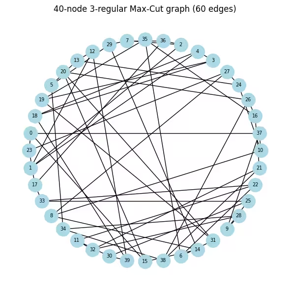
# ── Step 1a: Build the 40-node Max-Cut problem ─────────────────────────────
# A 3-regular graph (every node has exactly 3 neighbors) is a standard QAOA
N_LARGE = 40
G_large = nx.random_regular_graph(d=3, n=N_LARGE, seed=0)
edges_large = list(G_large.edges())
print(f"Graph: {N_LARGE} nodes, {len(edges_large)} edges (3-regular)")

# Visualize the graph so it is clear what problem we are solving before any
# quantum work. Nodes in a circular layout; each edge contributes +1 to the
# cut value when its endpoints land in different partitions.
pos_large = nx.circular_layout(G_large)
fig, ax = plt.subplots(figsize=(6, 6))
nx.draw(
    G_large,
    pos_large,
    with_labels=True,
    node_color="lightblue",
    node_size=400,
    font_size=7,
    ax=ax,
)
ax.set_title(f"40-node 3-regular Max-Cut graph ({len(edges_large)} edges)")
plt.tight_layout()
plt.show()

# Same Maxcut → OptimizationProblem → QUBO → Ising pipeline as the small example,
# applied to the 40-node graph.
prob_large = Maxcut(G_large).to_optimization_problem()
converter_large = OptimizationProblemToQubo()
qubo_large = converter_large.convert(prob_large)
cost_op_large, offset_large = to_ising(qubo_large)
n_qubits_large = cost_op_large.num_qubits
print(
    f"Cost operator: {n_qubits_large} qubits, {len(cost_op_large)} Pauli terms"
)

# ── Step 1b: QP relaxation (multi-start L-BFGS-B) ─────────────────────────
# Same multi-start approach as the small example. At 40 qubits the relaxed
# landscape has many more local minima, so 200 random starts are essential
# to find a low-energy warm-start point.
Q_large = qubo_large.objective.quadratic.to_array(symmetric=True)
mu_large = qubo_large.objective.linear.to_array()

def qp_obj_large(x):
    return x @ Q_large @ x + mu_large @ x + qubo_large.objective.constant

bounds_large = [(0.0, 1.0)] * n_qubits_large
rng_qp = np.random.default_rng(42)
best_val_large, c_star_large = np.inf, None

for _ in range(200):
    x0 = rng_qp.uniform(0.0, 1.0, n_qubits_large)
    res = minimize(qp_obj_large, x0, method="L-BFGS-B", bounds=bounds_large)
    if res.fun < best_val_large:
        best_val_large, c_star_large = res.fun, res.x

# Regularize and convert to rotation angles (same formula as small example)
epsilon_large = 0.25
c_clipped_large = np.clip(c_star_large, epsilon_large, 1 - epsilon_large)
thetas_large = 2 * np.arcsin(np.sqrt(c_clipped_large))
print(
    f"c* range: [{c_star_large.min():.3f}, {c_star_large.max():.3f}]  "
    f"theta range: [{thetas_large.min():.3f}, {thetas_large.max():.3f}] rad"
)

# Plot the distribution of c* values to see how much structure the relaxation
# extracted. Values near 0/1 mean confident assignments; values near 0.5 mean
# the classical solver was uncertain and quantum exploration is most needed there.
fig, ax = plt.subplots(figsize=(6, 3))
ax.hist(c_star_large, bins=20, color="steelblue", edgecolor="white")
ax.axvline(0.5, color="k", linestyle="--", label="Uniform prior (std QAOA)")
ax.set_xlabel(r"$c^*_i$")
ax.set_ylabel("Count")
ax.set_title(r"Distribution of warm-start values $c^*_i$ (40-node graph)")
ax.legend()
plt.tight_layout()
plt.show()

# ── Step 1c: Build WS-QAOA circuit ─────────────────────────────────────────
# Reuse build_ws_qaoa from the small-scale section unchanged; the helper
# scales automatically with n_qubits and the cost operator size.
p_large = 1
ws_qc_large, ws_gammas_large, ws_betas_large = build_ws_qaoa(
    cost_op_large, p_large, n_qubits_large, thetas_large
)
ws_qc_large.measure_all()

# ── Step 2: Transpile to hardware-native gates ──────────────────────────
# generate_preset_pass_manager compiles the abstract circuit to th
# gate set of the backend and inserts SWAP gates wherever the cost Hamiltonian
# couples qubits that are not directly connected on the processor.
pm = generate_preset_pass_manager(optimization_level=3, backend=backend)
ws_isa_large = pm.run(ws_qc_large)

ecr_count = ws_isa_large.count_ops().get("ecr", 0)
print(
    f"\nTranspiled circuit: 2Q depth={ws_isa_large.depth(lambda x: x.operation.num_qubits == 2)}"
)
ws_isa_large.draw("mpl", fold=-1)

Graph: 40 nodes, 60 edges (3-regular)

Cost operator: 40 qubits, 60 Pauli terms
c* range: [0.000, 1.000]  theta range: [1.047, 2.094] rad

Transpiled circuit: 2Q depth=86

# ── Classical baseline via simulated annealing ────────────────────
# Run SA before any hardware calls to get a strong classical reference cut
# value. SA is fast (seconds), needs no solver license, and reliably finds
# near-optimal solutions on 40-node graphs. We use sa_cut as the denominator
# for the approximation ratio instead of the looser QP upper bound.
#
# At each step we flip a random node and accept the move if it improves the
# cut, or with probability exp(delta/T) otherwise. Temperature T decays
# geometrically, allowing uphill moves early on to escape local minima.
def simulated_annealing_maxcut(
    G, seed=0, T0=2.0, T_min=1e-4, alpha=0.995, n_steps=100_000
):
    rng_sa = np.random.default_rng(seed)
    n = G.number_of_nodes()
    x = rng_sa.integers(0, 2, n)
    best_x = x.copy()
    best_cut = sum(1 for u, v in G.edges() if x[u] != x[v])
    T = T0
    for _ in range(n_steps):
        i = rng_sa.integers(0, n)
        delta = sum((-1 if x[i] != x[nb] else 1) for nb in G.neighbors(i))
        if delta > 0 or rng_sa.random() < np.exp(delta / T):
            x[i] ^= 1
            cut = sum(1 for u, v in G.edges() if x[u] != x[v])
            if cut > best_cut:
                best_cut, best_x = cut, x.copy()
        T = max(T * alpha, T_min)
    return best_x, best_cut

sa_solution, sa_cut = simulated_annealing_maxcut(G_large)
print(f"Simulated annealing cut value: {sa_cut}  (classical reference)")

# ── Step 3: Execution on hardware ───────────────────────────
# A Session reserves the backend so the COBYLA iterations and final sampling
# run back-to-back without re-queuing between jobs — important when the
# optimizer submits many short jobs sequentially. All jobs are tagged with
# "TUT_WSQAOA" for traceability in the IBM Quantum dashboard.
#
# EstimatorV2 with resilience_level=1 enables twirled readout error extinction
# (TREX), which corrects systematic measurement bit-flip errors without extra
# circuit overhead. 4096 shots per call balances estimation noise vs. job time.
estimator_options = EstimatorOptions()
estimator_options.resilience_level = 1
estimator_options.default_shots = 4096
estimator_options.environment.job_tags = ["TUT_WSQAOA"]

# Align the cost observable with the physical qubit layout chosen by the transpiler
cost_op_isa = cost_op_large.apply_layout(ws_isa_large.layout)
ws_param_order_isa = list(ws_isa_large.parameters)

ws_history_hw = []

with Session(backend=backend) as session:
    estimator_hw = Estimator(mode=session, options=estimator_options)

    def hw_cost_fn(params):
        bound = ws_isa_large.assign_parameters(
            dict(zip(ws_param_order_isa, params))
        )
        energy = (
            estimator_hw.run([(bound, cost_op_isa)]).result()[0].data.evs.real
        )
        ws_history_hw.append(float(energy))
        print(
            f"  iter {len(ws_history_hw):>3d}  <H_C> = {energy:.4f}", end="\r"
        )
        return float(energy)

    # Warm-start initialization: gamma=0 means the cost unitary is the identity on
    # the first call, so COBYLA immediately evaluates the warm-start state itself —
    # a much better starting signal than a random point.
    ws_params0_hw = np.concatenate(
        [np.zeros(p_large), np.full(p_large, np.pi / 4)]
    )

    ws_result_hw = minimize(
        hw_cost_fn,
        ws_params0_hw,
        method="COBYLA",
        options={"maxiter": 150, "rhobeg": 0.3},
    )
    print(
        f"\nOptimization complete: energy={ws_result_hw.fun:.4f}, "
        f"iterations={len(ws_history_hw)}"
    )

    # ── Step 3b: Sample the optimized circuit ──────────────────────────────────
    # Use 8192 shots for the final sample to get a reliable mode estimate.
    sampler_hw = Sampler(
        mode=session,
        options={"environment": {"job_tags": ["TUT_WSQAOA"]}},
    )
    ws_bound_hw = ws_isa_large.assign_parameters(
        dict(zip(ws_param_order_isa, ws_result_hw.x))
    )
    counts_hw = (
        sampler_hw.run([ws_bound_hw], shots=8192)
        .result()[0]
        .data.meas.get_counts()
    )

best_bs_hw = max(counts_hw, key=counts_hw.get)
best_count = counts_hw[best_bs_hw]
total_shots = sum(counts_hw.values())

# Decode: Qiskit returns bitstrings with qubit 0 at the rightmost position,
# so reversing the string maps character index i to variable x_i.
cut_val_hw, s0_hw, s1_hw = evaluate_cut(best_bs_hw[::-1], G_large)

# Compare against simulated annealing.
# A ratio >= 1.0 means WS-QAOA matched or beat the classical SA solution.
# A ratio close to 1.0 (e.g. > 0.95) shows the quantum result is competitive.
approx_ratio_hw = cut_val_hw / sa_cut
print(
    f"Most-probable bitstring frequency: {best_count}/{total_shots} "
    f"({100*best_count/total_shots:.1f}%)"
)
print(
    f"WS-QAOA cut: {cut_val_hw}  |  SA cut: {sa_cut}  "
    f"|  Approximation ratio vs SA: {approx_ratio_hw:.4f}"
)

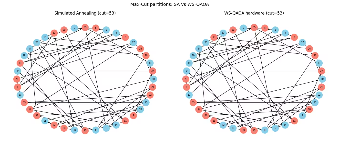
# Visualize both solutions side-by-side on the graph.
# Blue = partition S, orange = partition S-bar.
# Edges crossing between colors are the ones counted in the cut.
fig, axes = plt.subplots(1, 2, figsize=(14, 6))
for ax, assignment, cut, title in [
    (
        axes[0],
        list(sa_solution),
        sa_cut,
        f"Simulated Annealing (cut={sa_cut})",
    ),
    (
        axes[1],
        [int(b) for b in best_bs_hw[::-1]],
        cut_val_hw,
        f"WS-QAOA hardware (cut={cut_val_hw})",
    ),
]:
    colors = [
        "skyblue" if assignment[i] == 0 else "salmon" for i in G_large.nodes()
    ]
    nx.draw(
        G_large,
        pos_large,
        with_labels=True,
        node_color=colors,
        node_size=400,
        font_size=7,
        ax=ax,
    )
    ax.set_title(title)
plt.suptitle("Max-Cut partitions: SA vs WS-QAOA", fontsize=13)
plt.tight_layout()
plt.show()

# ── Step 4: Convergence plot and summary ──────────────────────────────────
# On real hardware the trace will be noisy (shot noise + gate errors), but the
# overall downward trend confirms that COBYLA is making progress despite noise.
fig, ax = plt.subplots(figsize=(7, 4))
ax.plot(ws_history_hw, color="tab:orange", label="WS-QAOA (hardware)")
ax.axhline(
    ws_result_hw.fun,
    color="tab:orange",
    linestyle=":",
    label=f"Final energy ({ws_result_hw.fun:.3f})",
)
ax.set_xlabel("Optimizer call")
ax.set_ylabel(r"$\langle H_C \rangle$")
ax.set_title(f"WS-QAOA convergence on {backend.name} (40 qubits, p=1)")
ax.legend()
plt.tight_layout()
plt.show()

print("\n=== Large Scale Summary ===")
print(f"{'Metric':<38} {'Value':>10}")
print("-" * 50)
print(f"{'Nodes / Edges':<38} {N_LARGE:>5} / {len(edges_large):<4}")
print(f"{'QAOA layers (p)':<38} {p_large:>10}")
print(f"{'Transpiled ECR gate count':<38} {ecr_count:>10}")
print(f"{'Transpiled circuit depth':<38} {ws_isa_large.depth():>10}")
print(f"{'Optimizer iterations':<38} {len(ws_history_hw):>10}")
print(f"{'WS-QAOA energy (hardware)':<38} {ws_result_hw.fun:>10.4f}")
print(f"{'Cut value':<38} {cut_val_hw:>10}")
print(f"{'Simulated annealing cut value':<38} {sa_cut:>10}")
print(f"{'Approximation ratio (vs SA)':<38} {approx_ratio_hw:>10.4f}")

Simulated annealing cut value: 53  (classical reference)
  iter  31  <H_C> = -12.4094
Optimization complete: energy=-13.0256, iterations=31
Most-probable bitstring frequency: 4/8192 (0.0%)
WS-QAOA cut: 53  |  SA cut: 53  |  Approximation ratio vs SA: 1.0000

=== Large Scale Summary ===
Metric                                      Value
--------------------------------------------------
Nodes / Edges                             40 / 60  
QAOA layers (p)                                 1
Transpiled ECR gate count                       0
Transpiled circuit depth                      276
Optimizer iterations                           31
WS-QAOA energy (hardware)                -13.0256
Cut value                                      53
Simulated annealing cut value                  53
Approximation ratio (vs SA)                1.0000

Mga Susunod na Hakbang

Recommendations

Kung interesado ka sa gawaing ito, maaaring interesado ka rin sa mga sumusunod na materyal:

• Mas mataas na QAOA layers: Dagdagan ang p para makita kung paano bumubuti ang parehong algorithm gamit ang mas maraming circuit layers, at kung nananatili ang bentahe ng WS-QAOA sa mababang depth.
• Qiskit addon optimization mapper: Tuklasin ang documentation at subukang i-model ang iba't ibang combinatorial problems, o gumamit ng iba't ibang solvers para sa continuous relaxation.

References

[1] D. J. Egger, J. Mareček, and S. Woerner, "Warm-starting quantum optimization," Quantum, vol. 5, p. 479, 2021. arXiv:2009.10095

[2] E. Farhi, J. Goldstone, and S. Gutmann, "A quantum approximate optimization algorithm," arXiv:1411.4028, 2014.