Gayahin ang neutron scattering sa mga quantum material gamit ang quantum circuits

Usage estimate: 13 minuto sa isang Heron r2 processor (TANDAAN: Ito ay tantiya lamang. Maaaring mag-iba ang iyong runtime.)

Aling tutorial ang dapat kong gamitin?

Gamitin ang tutorial na ito para matutunan ang implementation nang hakbang-hakbang, na may classical computation na tumatakbo nang lokal sa laptop mo at hardware execution sa isang IBM Quantum® QPU. Nangangailangan ng malaking memory ang large-scale na halimbawa, at ang approximate quantum compiling (AQC) ay maaaring tumagal ng ilang oras sa karaniwang resources ng laptop. Para ilipat ang compression sa Qiskit Serverless compute at memory resources, gamitin ang kasamang Serverless tutorial.

Mga learning outcome

Kung paano konektado ang inelastic neutron scattering (INS) spectra sa dynamical structure factors (DSFs) ng quantum spin models.
Kung paano maghanda ng ground state, maglapat ng lokal na perturbation, at magsagawa ng Trotter time evolution sa isang quantum circuit.
Kung paano gamitin ang approximate quantum compiling (AQC) gamit ang qiskit-addon-aqc-tensor upang i-compress ang malalalim na Trotter circuits para sa hardware execution.
Kung paano kunin ang retarded Green's function (RGF) mula sa qubit expectation values at i-Fourier-transform ito papunta sa isang DSF.

Prerequisites

Background

Sa tutorial na ito, nire-reproduce natin ang mga resulta ng Lee et al., arXiv:2603.15608.

Tinutulungan ng neutron scattering ang mga mananaliksik na i-characterize ang mga materyal na may kaugnayan sa sustainability, kabilang ang mga battery electrode. Sinusuri ng tutorial na ito kung paano maaaring i-simulate ng mga quantum circuit ang mga magnetic excitation at ikonekta ang mga theoretical model sa mga scattering measurement. Ang halimbawang quantum-magnet nito ay bumubuo ng mga paraan para sa pag-aaral ng material behavior, na nag-aambag sa mas malawak na research toolkit para sa materials discovery.

Inelastic neutron scattering at ang dynamical structure factor

Ang inelastic neutron scattering (INS) ay isa sa mga pinakamakapangyarihang experimental probe ng magnetic excitations sa quantum materials. Kapag tumama ang isang beam ng thermal o cold neutrons sa isang crystal, nagpapalitan ang mga indibidwal na neutron ng momentum $\mathbf{q}$ at enerhiyang $\omega$ kasama ang magnetic subsystem. Ang nasukat na scattering intensity ay proporsyonal sa dynamical structure factor (DSF),

$S^{\alpha\beta}(q,\omega) = \sum_{j} e^{-iq\,j}\int_{-\infty}^{\infty} dt\; e^{i\omega t}\, \langle S_0^{\alpha}(0)\, S_j^{\beta}(t)\rangle,$

na naglalaman ng buong space-time correlations ng mga spin degrees of freedom.

KCuF $_3$ : isang canonical na Luttinger-liquid magnet

Ang potassium copper fluoride (KCuF $_3$ ) ay isang quasi-one-dimensional antiferromagnet kung saan ang mga chain ng spin- $\frac{1}{2}$ Cu $^{2+}$ ions ay nakikipag-interact sa pamamagitan ng nearest-neighbor Heisenberg exchange $J$ , habang ang interchain coupling ay $\sim 2.7\%$ lamang ng $J$ . Sa $T = 6\;\mathrm{K}$ kung saan available ang INS data, ang spectrum ay dominado ng fractionalized spinon excitations na katangian ng isang Tomonaga-Luttinger liquid. Dahil ang intrachain dynamics ay mahusay na inilalarawan ng one-dimensional spin- $\frac{1}{2}$ XXZ Hamiltonian sa isotropic point ( $\epsilon = 1$ ),

$H = J\sum_{i}\left[S_i^Z S_{i+1}^Z + \epsilon\left(S_i^X S_{i+1}^X + S_i^Y S_{i+1}^Y\right)\right],$

Ang KCuF $_3$ ay nagsisilbing isang ideal na benchmark para sa quantum simulation: sapat na simple ang Hamiltonian upang maipatupad sa isang quantum processor, ngunit ang ground state ay lubos na entangled at ang excitation spectrum ay nagtataglay ng malawak na two-spinon continuum.

Tandaan: itinatakda ng tutorial na ito ang $J = 1$ bilang unit ng enerhiya at ginagamit ang normalization na $H = J\sum_i[\ldots]$ , na katumbas ng local Hamiltonian na $H_\mathrm{loc} = J(S^X S^X + S^Y S^Y + S^Z S^Z)$ na ginamit sa circuit implementation ng papel (Fig. S3 ng supplementary). Ang buong Hamiltonian ng papel (Eq. 3) ay may karagdagang overall factor na 2, kaya ang $J$ ng papel ay doble ng $J$ na ginamit dito.

Ano ang aming sinisimulate at sinusukat

Ang pisikal na dami na kinakalkula natin ay ang retarded Green's function (RGF), na tinukoy bilang ang time-dependent spin-spin correlation function

$G^R_{\alpha,\beta}(j, j_c, t) = -\frac{i}{2}\,\langle\psi_{\mathrm{GS}}|\,S_j^\alpha(t)\,S_{j_c}^\beta(0) - S_{j_c}^\beta(0)\,S_j^\alpha(t)\,|\psi_{\mathrm{GS}}\rangle,$

kung saan ang $j_c$ ay isang reference site (ang gitna ng chain) at ang $S_j^\alpha(t) = e^{iHt}S_j^\alpha e^{-iHt}$ ay ang Heisenberg-picture spin operator. Sa tutorial na ito, nakatuon tayo sa $zz$ component ( $\alpha = \beta = z$ ). Sa isang quantum computer, naa-access ang RGF sa pamamagitan ng paghahanda ng ground state, paglalapat ng lokal na perturbation sa $j_c$ , time-evolving ng na-perturb na state, at pagsukat ng single-qubit expectation value na $\langle\sigma_j^z\rangle$ sa bawat site $j$ para sa bawat time step. Ang mahalagang insight ay ang bawat $\langle\sigma_j^z\rangle$ ay nagbibigay ng pagkakaiba mula sa ground-state magnetization; dahil ang isotropic Heisenberg antiferromagnet ay may zero net per-site magnetization ( $\langle\sigma_j^z\rangle_\mathrm{GS} = 0$ ), direktang nagbubunga ang hilaw na sinukat na halaga ng $G^R(j, j_c, t)$ nang walang anumang explicit na pagbabawas.

Sa pamamagitan ng pagkolekta ng $G^R(j, j_c, t)$ sa lahat ng sites at time steps, binubuo natin ang isang two-dimensional dataset na pagkatapos ay Fourier-transformed sa parehong espasyo at oras upang makabuo ng dynamical structure factor $S(q,\omega)$ . Ang DSF ang dami na direktang sinusukat sa isang INS experiment: sinasabi nito sa atin kung anong magnetic excitations ang umiiral sa bawat momentum $q$ at enerhiyang $\omega$ . Para sa isotropic Heisenberg chain, ang eksaktong excitation spectrum ay isang two-spinon continuum, isang malawak na band ng scattering intensity kung saan ang hugis nito ay nagsisilbing mahigpit na end-to-end benchmark para sa quantum simulation: pinapatunayan nito ang ground-state preparation, perturbation, Trotter time evolution, at measurement protocol nang sabay-sabay.

Workflow ng quantum simulation

Ginagaya ng workflow ang pisika ng isang INS event. Tayo ay (1) naghahanda ng many-body ground state $|\psi_{\mathrm{GS}}\rangle$ sa $n$ qubits, (2) naglalapat ng lokal na spin-flip perturbation $U_{j_c} = \frac{1}{\sqrt{2}}(I - i\sigma^z_{j_c})$ sa gitna ng chain upang gayahin ang spin transfer ng neutron, (3) nag-eebolba sa ilalim ng $H$ para sa discrete time steps gamit ang second-order Trotterization, at (4) sinusukat ang $\langle\sigma_i^z\rangle$ sa bawat qubit sa bawat step upang makuha ang RGF. Pagkatapos, nagbubunga ng DSF na $S(q,\omega)$ ang isang two-dimensional discrete Fourier transform.

Ang observable na sinusukat natin sa bawat time step ay ang $\sigma_i^z$ sa bawat qubit $i$ . Sa Qiskit, ito ay kinakatawan bilang isang listahan ng SparsePauliOp operators: isang single-qubit $Z$ na naka-embed sa $n$ -qubit identity string para sa bawat site. Binubuo nang isang beses lamang ang mga observable na ito sa bawat problem instance sa panahon ng problem-mapping step (Step 1) at muling ginagamit para sa bawat circuit sa sukat na iyon.

Approximate quantum compiling (AQC)

Ang malalalim na Trotter circuits ay maaaring i-compress gamit ang approximate quantum compiling (AQC), na pinapalitan ang unang ilang Trotter layers ng isang mas maikling parameterized ansatz kung saan ang mga parameter nito ay classically optimized upang i-maximize ang MPS-level fidelity kasama ang orihinal na malalim na circuit. Ang natitirang mga Trotter step ay eksaktong idinaragdag, na gumagawa ng isang "mixed" AQC + Trotter circuit na may malaking bawas na two-qubit gates.

Simulation ng MPS

Para sa isang one-dimensional na sistema, ang matrix-product-state (MPS) methods ay mahusay na nakapag-simulate ng parehong ground-state preparation (gamit ang density matrix renormalization group, o DMRG) at circuit-level time evolution. Sa pamamagitan ng pagkontrol sa bond dimension $\chi$ , ipinagpapalit natin ang accuracy laban sa computational cost. Sa tutorial na ito, gumagamit tayo ng MPS simulation sa loob ng qiskit-addon-aqc-tensor upang kalkulahin ang high-fidelity AQC ansätze na nagko-compress ng malalalim na Trotter circuits para sa hardware execution.

Requirements

Bago simulan ang tutorial na ito, siguraduhing naka-install ang mga sumusunod:

Qiskit SDK na may suporta sa visualization
Qiskit Runtime (pip install qiskit-ibm-runtime)
qiskit-addon-aqc-tensor na may quimb at JAX extras (pip install 'qiskit-addon-aqc-tensor[quimb-jax]')

Setup

# Added by doQumentation — installs the packages this notebook needs if they are missing
import importlib.util

_needed = {"matplotlib": "matplotlib", "numpy": "numpy", "qiskit": "qiskit", "qiskit_addon_aqc_tensor": "qiskit-addon-aqc-tensor", "qiskit_ibm_runtime": "qiskit-ibm-runtime", "qiskit_quimb": "qiskit-quimb", "quimb": "quimb", "scipy": "scipy"}
_missing = [pip for module, pip in _needed.items()
            if importlib.util.find_spec(module) is None]
# One at a time, so a package that fails to install does not block the others
for _pip in _missing:
    %pip install -q {_pip}
if not _missing:
    print("\u2713 All required packages are installed")

import timeit
import warnings
from collections.abc import Iterator, Sequence
from functools import partial

import matplotlib.pyplot as plt
import numpy as np
import quimb.tensor as qtn
import scipy.optimize
from numpy.typing import NDArray
from qiskit import QuantumCircuit
from qiskit.circuit import CircuitInstruction, ParameterVector, Qubit
from qiskit.circuit.library import PauliEvolutionGate
from qiskit.primitives import StatevectorEstimator
from qiskit.quantum_info import SparsePauliOp
from qiskit.transpiler.preset_passmanagers import generate_preset_pass_manager
from qiskit_addon_aqc_tensor import generate_ansatz_from_circuit
from qiskit_addon_aqc_tensor.objective import MaximizeStateFidelity
from qiskit_addon_aqc_tensor.simulation import tensornetwork_from_circuit
from qiskit_addon_aqc_tensor.simulation.quimb import QuimbSimulator
from qiskit_ibm_runtime import EstimatorV2 as Estimator
from qiskit_ibm_runtime import QiskitRuntimeService
from qiskit_quimb import quimb_circuit
from scipy.sparse import SparseEfficiencyWarning

# scipy.sparse.linalg.expm (reached via PauliEvolutionGate.to_matrix) prefers
# CSC and warns when handed the CSR matrix from SparsePauliOp.to_matrix; the
# result is unaffected, so silence the cosmetic warning.
warnings.filterwarnings("ignore", category=SparseEfficiencyWarning)

def xxz_hamiltonian_mpo(
    n_qubits: int, interaction: float = 1.0, anisotropy: float = 1.0
) -> qtn.MatrixProductOperator:
    """1D XXZ Hamiltonian as a quimb MPO.

    Builds the Hamiltonian using ``qtn.SpinHam1D``.

    Args:
        n_qubits: Number of sites.
        interaction: Overall interaction strength (J in the paper).
        anisotropy: XY/Z anisotropy (ε in the paper). ``ε = 1`` is the
            isotropic Heisenberg point; ``ε = 0`` is the Ising limit.

    Returns:
        The Hamiltonian as a matrix product operator.
    """
    builder = qtn.SpinHam1D(S=1 / 2)
    builder += interaction * anisotropy * 0.5, "+", "-"
    builder += interaction * anisotropy * 0.5, "-", "+"
    builder += interaction, "Z", "Z"
    return builder.build_mpo(L=n_qubits)

def build_ground_state_ansatz(n_qubits: int, n_layers: int) -> QuantumCircuit:
    """Hamiltonian variational ansatz (HVA) circuit for ground-state preparation.

    Starts from a product of singlet pairs and applies alternating
    odd/even layers of parameterized XXZ pair-evolution gates.

    The returned circuit is parameterized: it carries a ``ParameterVector``
    named ``"theta"`` of length ``2 * n_layers`` whose values must be
    assigned (e.g. via ``circuit.assign_parameters``) before simulation.
    Element ``2 * r`` is the odd-layer angle and element ``2 * r + 1`` is the
    even-layer angle of layer ``r``.

    Args:
        n_qubits: Number of qubits (must be even).
        n_layers: Number of HVA layers.

    Returns:
        The parameterized HVA preparation circuit.
    """
    theta = ParameterVector("theta", 2 * n_layers)
    circuit = QuantumCircuit(n_qubits)
    # Initial singlet product state
    for i in range(n_qubits // 2):
        circuit.x(2 * i)
        circuit.x(2 * i + 1)
        circuit.h(2 * i + 1)
        circuit.cx(2 * i + 1, 2 * i)
    # Variational layers: each pair gate is exp(-i theta (XX+YY+ZZ)/2)
    pair_ham = SparsePauliOp(
        ["XX", "YY", "ZZ"], coeffs=[0.5, 0.5, 0.5]
    )  # H_pair (HVA form)
    for r in range(n_layers):
        for i in range(1, (n_qubits + 1) // 2):  # odd layer
            circuit.append(
                PauliEvolutionGate(pair_ham, time=theta[2 * r]),
                [2 * i - 1, 2 * i],
            )
        for i in range(n_qubits // 2):  # even layer
            circuit.append(
                PauliEvolutionGate(pair_ham, time=theta[2 * r + 1]),
                [2 * i, 2 * i + 1],
            )
    return circuit

def optimize_ground_state_ansatz(
    ansatz: QuantumCircuit,
    x0: NDArray[np.floating],
    target_mps: qtn.MatrixProductState,
    *,
    max_bond: int | None = None,
    cutoff: float = 1e-10,
    method: str = "COBYQA",
    options: dict | None = None,
) -> scipy.optimize.OptimizeResult:
    """Optimize HVA parameters by maximizing fidelity with a target MPS.

    The HVA circuit is simulated as a matrix product state with the given
    bond-dimension truncation, and the parameters are optimized to maximize
    the state fidelity ``|<psi_HVA | target_mps>|**2`` with the DMRG ground
    state. Both states are normalized, so the minimized objective is the
    infidelity ``1 - |<psi_HVA | target_mps>|**2``.

    Args:
        ansatz: Parameterized HVA circuit from ``build_ground_state_ansatz``.
            The length of ``x0`` must equal ``ansatz.num_parameters``.
        x0: Initial parameters.
        target_mps: Target MPS (DMRG ground state) to maximize fidelity with.
        max_bond: Maximum MPS bond dimension during gate application.
        cutoff: Singular-value cutoff during gate application.
        method: ``scipy.optimize.minimize`` method.
        options: Options dict forwarded to ``scipy.optimize.minimize``.

    Returns:
        The Scipy OptimizeResult.
    """

    def infidelity(params: NDArray[np.floating]) -> float:
        circuit = ansatz.assign_parameters(params)
        circuit_mps = quimb_circuit(
            circuit.decompose(["PauliEvolution"]),
            quimb_circuit_class=qtn.CircuitMPS,
            max_bond=max_bond,
            cutoff=cutoff,
        )
        return 1 - abs(circuit_mps.psi.H @ target_mps) ** 2

    return scipy.optimize.minimize(
        infidelity, np.asarray(x0), method=method, options=options
    )

def trotter_evolution(
    qubits: Sequence[Qubit],
    interaction: float,
    anisotropy: float,
    time_step: float,
    n_steps: int,
) -> Iterator[CircuitInstruction]:
    """Second-order Trotter steps of the XXZ pair Hamiltonian.

    While the paper used a hand-optimized circuit for the Trotter steps, we use
    PauliEvolutionGate here for simplicity and generality. The final two-qubit gate
    count and gate depth are equivalent when transpiled with ``optimization_level=3``.

    Args:
        qubits: Qubits to act on (length ``n_qubits``).
        interaction: Overall interaction strength (J in the paper).
        anisotropy: XY/Z anisotropy (ε in the paper). ``ε = 1`` is the
            isotropic Heisenberg point; ``ε = 0`` is the Ising limit.
        time_step: Per-step Trotter time.
        n_steps: Number of Trotter steps.

    Yields:
        ``CircuitInstruction``s implementing the Trotter steps.
    """
    if n_steps == 0:
        return
    n_qubits = len(qubits)
    pair_ham = SparsePauliOp(
        ["XX", "YY", "ZZ"],
        coeffs=[
            0.25 * interaction * anisotropy,
            0.25 * interaction * anisotropy,
            0.25 * interaction,
        ],
    )
    half_evo = PauliEvolutionGate(pair_ham, time=time_step / 2)
    full_evo = PauliEvolutionGate(pair_ham, time=time_step)
    for i in range(n_qubits // 2):  # half even layer
        yield CircuitInstruction(half_evo, (qubits[2 * i], qubits[2 * i + 1]))
    for i in range(n_qubits // 2 - 1):  # full odd layer
        yield CircuitInstruction(
            full_evo, (qubits[2 * i + 1], qubits[2 * i + 2])
        )
    for _ in range(n_steps - 1):  # interior steps
        for i in range(n_qubits // 2):
            yield CircuitInstruction(
                full_evo, (qubits[2 * i], qubits[2 * i + 1])
            )
        for i in range(n_qubits // 2 - 1):
            yield CircuitInstruction(
                full_evo, (qubits[2 * i + 1], qubits[2 * i + 2])
            )
    for i in range(n_qubits // 2):  # half even layer
        yield CircuitInstruction(half_evo, (qubits[2 * i], qubits[2 * i + 1]))

def get_dsf(
    n_qubits: int,
    rgf_mat: NDArray[np.floating],
    time_step: float,
    n_steps: int,
    n_points_momentum: int,
    n_points_frequency: int,
) -> NDArray[np.floating]:
    """Compute the dynamical structure factor from the retarded Green's function.

    Uses the center-site approximation and a discrete Fourier transform.
    The result is symmetrized about the momentum axis and clipped to
    non-negative values, ready for plotting.

    Args:
        n_qubits: Number of qubits (sites).
        rgf_mat: RGF matrix of shape ``(n_steps, n_qubits)``.
        time_step: Trotter time-step size.
        n_steps: Number of time steps.
        n_points_momentum: Number of momentum points.
        n_points_frequency: Number of frequency points.

    Returns:
        DSF array of shape ``(n_points_frequency, n_points_momentum)``,
        symmetrized about the momentum axis and clipped to non-negative values.
    """
    max_frequency = np.pi / time_step
    momentum_range = np.linspace(0, 2 * np.pi, n_points_momentum)
    frequency_range = np.linspace(0, max_frequency, n_points_frequency)
    result = np.zeros((frequency_range.shape[0], momentum_range.shape[0]))
    center = n_qubits // 2 - 1
    for iw, w in enumerate(frequency_range):
        exponent = np.exp(1j * w * time_step * np.arange(1, n_steps + 1))
        # S = sigma/2, so two spin operators contribute a factor of (1/2)(1/2) = 1/4.
        rgf_omega = (
            np.dot(rgf_mat.T, exponent) * time_step / 4
        )  # S(omega): time Fourier slice of the Green's function
        for iq, q in enumerate(momentum_range):
            momentum_phases = np.exp(
                -1j * q * np.arange(-center, center + 2, 1)
            )
            result[iw, iq] = np.imag(np.dot(rgf_omega, momentum_phases))
    result = -(result + result[:, ::-1]) / 2
    result = np.clip(result, a_min=0, a_max=None)
    return result

def plot_dsf(
    dsf: NDArray[np.floating],
    time_step: float,
    n_points_momentum: int,
    n_points_frequency: int,
    title: str | None = None,
) -> None:
    """Heat-map of the dynamical structure factor.

    Args:
        dsf: DSF array of shape ``(n_points_frequency, n_points_momentum)``.
        time_step: Trotter time-step size.
        n_points_momentum: Number of momentum points.
        n_points_frequency: Number of frequency points.
        title: Optional plot title.
    """
    max_frequency = np.pi / time_step
    momentum_range = np.linspace(0, 2 * np.pi, n_points_momentum)
    frequency_range = np.linspace(0, max_frequency, n_points_frequency)
    x, y = np.meshgrid(momentum_range, frequency_range)
    fig, ax = plt.subplots(figsize=(8, 5))
    c = ax.pcolormesh(x, y, dsf / np.max(dsf), cmap="viridis", shading="auto")
    fig.colorbar(c, ax=ax, label="Normalized intensity")
    ax.set_ylim(0, 3.6)
    ax.set_xlim(0, 2 * np.pi)
    ax.set_xlabel(r"$q$", fontsize=16)
    ax.set_ylabel(r"$\tilde{\omega} = \omega / J$", fontsize=16)
    ax.set_xticks([0, np.pi / 2, np.pi, 3 * np.pi / 2, 2 * np.pi])
    ax.set_xticklabels(["0", r"$\pi/2$", r"$\pi$", r"$3\pi/2$", r"$2\pi$"])
    if title:
        ax.set_title(title, fontsize=14)
    plt.tight_layout()
    plt.show()

def plot_rgf(
    n_qubits: int,
    rgf_mat: NDArray[np.floating],
    time_step: float,
    n_steps: int,
    title: str | None = None,
) -> None:
    """Heat-map of the retarded Green's function in real space and time.

    Args:
        n_qubits: Number of qubits (sites).
        rgf_mat: RGF matrix of shape ``(n_steps, n_qubits)``.
        time_step: Trotter time-step size.
        n_steps: Number of time steps.
        title: Optional plot title.
    """
    fig, ax = plt.subplots(figsize=(8, 6))
    qubit_axis = np.arange(n_qubits)
    t_axis = np.arange(1, n_steps + 1) * time_step
    x, y = np.meshgrid(qubit_axis, t_axis)
    c = ax.pcolormesh(
        x,
        y,
        np.real(rgf_mat),
        cmap="RdBu",
        vmax=0.5,
        vmin=-0.5,
        shading="auto",
    )
    fig.colorbar(c, ax=ax, label=r"Re $G^R(j, j_c, t)$")
    ax.set_xlabel("Qubit", fontsize=16)
    ax.xaxis.set_major_locator(
        plt.matplotlib.ticker.MaxNLocator(integer=True)
    )
    ax.set_ylabel(r"Time", fontsize=16)
    if title:
        ax.set_title(title, fontsize=14)
    plt.tight_layout()
    plt.show()

def uniform_2q_depth(circuit: QuantumCircuit) -> int:
    """Two-qubit gate depth in a standardized basis."""
    pass_manager = generate_preset_pass_manager(
        optimization_level=0, basis_gates=["cz", "id", "rz", "sx", "x"]
    )
    return pass_manager.run(circuit).depth(
        lambda inst: inst.operation.num_qubits == 2
    )

Halimbawa ng simulator sa maliit na sukat

Una nating ipinapakita ang buong workflow sa 10 qubits, ino-optimize ang HVA ground-state ansatz gamit ang MPS simulation at ginagamit ang Qiskit statevector simulator para sa time evolution. Nagbibigay ang DMRG ng reference ground-state energy at isang reference MPS. Ang maliit na halimbawang ito ay nagbibigay-daan sa atin na patunayan ang bawat hakbang bago mag-scale up.

Step 1: I-map ang mga classical input sa isang quantum problem

Nagsisimula tayo sa pagtukoy ng pisikal na modelo at pagbuo ng quantum circuits.

Hamiltonian. Ang KCuF $_3$ ay minomodelo ng 1D XXZ Hamiltonian sa isotropic point ( $J = 1$ , $\epsilon = 1$ , itinatakda ang $J = 1$ bilang unit ng enerhiya).

Ground state. Gumagamit tayo ng isang Hamiltonian variational ansatz (HVA) circuit, build_ground_state_ansatz, bilang ground-state preparation circuit. Ang mga HVA parameter ay classically optimized sa pamamagitan ng pag-maximize ng state fidelity na $|\langle\psi_{\mathrm{HVA}}(\theta)|\psi_{\mathrm{DMRG}}\rangle|^2$ kasama ang DMRG ground-state MPS, kung saan ang HVA state ay sinusuri sa pamamagitan ng pag-simulate ng circuit bilang matrix product state gamit ang CircuitMPS ng quimb. Ginagamit natin ang scipy.optimize.minimize para sa optimization. Ang enerhiyang $\langle H \rangle$ ng na-optimize na ansatz ay kinakalkula rin bilang reference.

Trotter gates. Ang bawat nearest-neighbor interaction term na $e^{-i\Delta t\, H_{\mathrm{pair}}}$ na may $H_{\mathrm{pair}} = (J/4)(XX + YY + ZZ)$ ay binubuo gamit ang PauliEvolutionGate(H_pair, time=time_step). Sini-synthesize ito ng Qiskit sa optimal na three-CNOT decomposition sa panahon ng transpilation.

Perturbation. Isang $R_z(\pi/2)$ gate sa gitnang qubit ang nagpapatupad ng $U_{j_c} = \frac{1}{\sqrt{2}}(I - i\sigma^z_{j_c})$ , na ginagaya ang lokal na spin-flip na ginagawa ng isang scattered neutron.

Observables. Bumubuo tayo ng $\sigma^z$ observable para sa bawat qubit site. Ang mga SparsePauliOp object na ito ay ipinapasa sa Estimator primitive sa Step 3 upang makuha ang $\langle\sigma_i^z\rangle$ sa bawat time step.

# -- Physical parameters --
n_qubits = 10
interaction = 1.0  # J
anisotropy = 1.0  # ε (isotropic point)
time_step = 0.6
n_steps = 10
mps_max_bond = 32
mps_cutoff = 1e-8
center = n_qubits // 2 - 1

# -- Hamiltonian MPO --
ham_mpo = xxz_hamiltonian_mpo(n_qubits, interaction, anisotropy)

# -- Reference ground-state energy via DMRG --
dmrg = qtn.DMRG2(ham_mpo)
dmrg.solve(tol=1e-8)
print(f"Ground-state energy (DMRG): {dmrg.energy:.6f}")

# -- Build ground state ansatz circuit --
gs_n_layers = 3
gs_ansatz = build_ground_state_ansatz(n_qubits, gs_n_layers)

# -- Optimize ground state ansatz parameters to maximize fidelity with the DMRG MPS --
# Initialize odd-layer angles near 0 (where the inter-pair gate is the
# identity) and even-layer angles near pi/2 (where the intra-pair gate
# is a SWAP, since 0.5*(XX + YY + ZZ) = SWAP - I/2).
rng = np.random.default_rng(12345)
x0 = np.tile([0, np.pi / 2], gs_n_layers) + rng.normal(
    scale=0.1, size=2 * gs_n_layers
)
print("Optimizing ground state ansatz...")
t0 = timeit.default_timer()
result = optimize_ground_state_ansatz(
    gs_ansatz,
    x0,
    dmrg.state,
    max_bond=mps_max_bond,
    cutoff=mps_cutoff,
    options=dict(maxiter=100),
)
t1 = timeit.default_timer()
print(f"Finished optimizing ground state ansatz in {t1 - t0} seconds.")
print(f"Ground state ansatz fidelity: {1 - result.fun:.6f}")

gs_circuit = gs_ansatz.assign_parameters(result.x)
gs_circuit_mps = quimb_circuit(
    gs_circuit.decompose(["PauliEvolution"]),
    quimb_circuit_class=qtn.CircuitMPS,
    max_bond=mps_max_bond,
    cutoff=mps_cutoff,
)
gs_ansatz_energy = qtn.expec_TN_1D(
    gs_circuit_mps.psi.H, ham_mpo, gs_circuit_mps.psi
)
print(f"Ground state ansatz energy: {gs_ansatz_energy:.6f}")

# -- Build circuits for each time step --
perturbed = gs_circuit.copy()
perturbed.rz(np.pi / 2, center)

circuits = []
for t in range(1, n_steps + 1):
    circuit = perturbed.copy()
    for instr in trotter_evolution(
        circuit.qubits, interaction, anisotropy, time_step, t
    ):
        circuit.append(instr)
    circuits.append(circuit)
print(
    f"Built {len(circuits)} circuits, deepest 2q depth (uniform basis) = "
    f"{uniform_2q_depth(circuits[-1])}"
)

# -- Observables: Z on each qubit site --
observables = [
    SparsePauliOp.from_sparse_list([("Z", [i], 1)], num_qubits=n_qubits)
    for i in range(n_qubits)
]
print(f"Defined {len(observables)} Z observables.")

Ground-state energy (DMRG): -4.258035
Optimizing ground state ansatz...
Finished optimizing ground state ansatz in 8.850687621976249 seconds.
Ground state ansatz fidelity: 0.984277
Ground state ansatz energy: -4.232565
Built 10 circuits, deepest 2q depth (uniform basis) = 163
Defined 10 Z observables.

Step 2: I-optimize ang problema para sa pagpapatakbo sa quantum hardware

Para sa aktwal na hardware, ang mga Trotter circuits sa itaas ay masyadong malalim. Ang approximate quantum compiling (AQC) ay tumutugon dito sa pamamagitan ng pagpalit sa unang $k$ Trotter layers (kasama ang ground-state circuit) ng isang mas maikling parameterized ansatz na na-optimize upang i-maximize ang MPS-level fidelity kasama ang orihinal na malalim na circuit. Ang natitirang mga Trotter step ay eksaktong idinaragdag, na gumagawa ng mas mababaw na "AQC + Trotter" circuit.

Upang balansehin ang expressibility laban sa lalim ng circuit, dalawang ansätze ang ginagamit: ang isang one-layer ansatz (nabuo mula sa isang Trotter step) ay nagko-compress ng pinakaunang time steps, at ang mas malalim na two-layer ansatz (nabuo mula sa dalawang Trotter step) ay nagko-compress ng susunod na ilang steps kung saan kailangan ang mas mataas na fidelity.

Ang AQC workflow ay may apat na sub-step:

Bumuo ng target circuits — ang unang $k_1 + k_2$ circuits mula sa Step 1 ay direktang nagsisilbing AQC targets.
Kalkulahin ang target MPS — i-simulate ang bawat target circuit bilang matrix-product state gamit ang quimb.tensor.CircuitMPS.
Bumuo at i-optimize ang mga ansätze — gumagawa ang generate_ansatz_from_circuit ng isang one-layer at isang two-layer na parameterized ansatz; ang mga parameter ay na-optimize gamit ang L-BFGS-B na may JAX-accelerated gradients upang i-minimize ang $1 - |\langle\psi_{\mathrm{ansatz}}|\psi_{\mathrm{target}}\rangle|^2$ . Ang unang $k_1$ steps ay gumagamit ng one-layer ansatz at ang susunod na $k_2$ steps ay gumagamit ng two-layer ansatz; sa loob ng bawat stage, nagwa-warm-start ang bawat step mula sa na-optimize na parameters ng naunang step, at nire-reset ang mga parameter sa stage defaults sa hangganan ng stage.
Buuin ang mixed circuits — para sa time steps lampas sa AQC checkpoint, idinaragdag ang eksaktong Trotter layers sa na-optimize na two-layer AQC circuit gamit ang trotter_evolution.

# Number of time steps to compress into an AQC ansatz with one layer
aqc_n_steps_1 = 3
# Number of time steps to compress into an AQC ansatz with two layers
aqc_n_steps_2 = 2
aqc_n_steps_total = aqc_n_steps_1 + aqc_n_steps_2

# ── Step 2a: Target circuits (first aqc_n_steps_total circuits from Step 1) ──
target_circuits = {
    k: circuits[k - 1] for k in range(1, aqc_n_steps_total + 1)
}
# ── Step 2b: Compute target MPS ──
# Decompose PauliEvolutionGate to RXX/RYY/RZZ before passing to the AQC MPS
# backend, which does not understand PauliEvolutionGate natively.
aqc_sim = QuimbSimulator(
    quimb_circuit_factory=partial(
        qtn.CircuitMPS,
        gate_opts=dict(max_bond=mps_max_bond, cutoff=mps_cutoff),
    ),
    autodiff_backend="jax",
)
print("\nStep 2b — target MPS:")
target_mps = {}
for k in range(1, aqc_n_steps_total + 1):
    target_mps[k] = tensornetwork_from_circuit(
        target_circuits[k].decompose(["PauliEvolution"]), aqc_sim
    )
    print(f"  k={k}: max bond = {target_mps[k].psi.max_bond()}")

# ── Step 2c: Generate ansätze (one-layer and two-layer) and optimize parameters ──
ansatz_1, initial_params_1 = generate_ansatz_from_circuit(
    target_circuits[1].decompose(["PauliEvolution"]),
    qubits_initially_zero=True,
)
initial_params_1 = np.array(initial_params_1)
ansatz_2, initial_params_2 = generate_ansatz_from_circuit(
    target_circuits[2].decompose(["PauliEvolution"]),
    qubits_initially_zero=True,
)
initial_params_2 = np.array(initial_params_2)
print(
    f"\nStep 2c — one-layer ansatz: {ansatz_1.num_parameters} parameters, "
    f"2q depth (uniform basis) = {uniform_2q_depth(ansatz_1)}"
)
print(
    f"Step 2c — two-layer ansatz: {ansatz_2.num_parameters} parameters, "
    f"2q depth (uniform basis) = {uniform_2q_depth(ansatz_2)}"
)

aqc_circuits = {}
aqc_params = {}
for k in range(1, aqc_n_steps_total + 1):
    if k <= aqc_n_steps_1:
        ansatz, base_params = ansatz_1, initial_params_1
    else:
        ansatz, base_params = ansatz_2, initial_params_2
    # Warm-start from the previous step only within the same stage
    same_stage = (k - 1 >= 1) and (
        (k - 1 <= aqc_n_steps_1) == (k <= aqc_n_steps_1)
    )
    x0 = aqc_params[k - 1] if same_stage else base_params
    obj = MaximizeStateFidelity(target_mps[k], ansatz, aqc_sim)
    t0 = timeit.default_timer()
    result = scipy.optimize.minimize(
        obj.loss_function,
        x0,
        method="L-BFGS-B",
        jac=True,
        options=dict(maxiter=100),
    )
    elapsed = timeit.default_timer() - t0
    aqc_params[k] = result.x
    aqc_circuits[k] = ansatz.assign_parameters(result.x)
    print(
        f"  k={k}: fidelity = {1 - result.fun:.4f}, "
        f"2q depth (uniform basis) = "
        f"{uniform_2q_depth(aqc_circuits[k])}, "
        f"{elapsed:.1f}s"
    )

# ── Step 2d: Assemble full circuit set (AQC + Trotter) ──
all_circuits = []
for k in range(1, aqc_n_steps_total + 1):
    all_circuits.append(aqc_circuits[k])
base = aqc_circuits[aqc_n_steps_total]
for k in range(1, n_steps - aqc_n_steps_total + 1):
    circuit = base.copy()
    for instr in trotter_evolution(
        circuit.qubits, interaction, anisotropy, time_step, k
    ):
        circuit.append(instr)
    all_circuits.append(circuit)

full_depths = [
    uniform_2q_depth(circuits[k - 1]) for k in range(1, n_steps + 1)
]
aqc_depths = [uniform_2q_depth(circuit) for circuit in all_circuits]
full_2q = [
    circuits[k - 1].decompose(["PauliEvolution"]).num_nonlocal_gates()
    for k in range(1, n_steps + 1)
]
aqc_2q = [
    circuit.decompose(["PauliEvolution"]).num_nonlocal_gates()
    for circuit in all_circuits
]
print(f"\nStep 2d — assembled {len(all_circuits)} circuits")
print(
    f"  At step {n_steps} (uniform basis): "
    f"Trotter 2q depth = {full_depths[-1]}, AQC+Trotter 2q depth = {aqc_depths[-1]}; "
    f"2q gates: Trotter = {full_2q[-1]}, AQC+Trotter = {aqc_2q[-1]}"
)

steps_axis = np.arange(1, n_steps + 1)
fig, ax = plt.subplots(figsize=(7, 4))
ax.plot(steps_axis, full_depths, "-o", color="black", label="Full Trotter")
ax.plot(
    steps_axis, aqc_depths, "-o", color="cadetblue", label="AQC + Trotter"
)
ax.set_xlabel("Trotter steps", fontsize=13)
ax.xaxis.set_major_locator(plt.matplotlib.ticker.MaxNLocator(integer=True))
ax.set_ylabel("2q gate depth (uniform basis)", fontsize=13)
ax.set_title(f"AQC circuit-depth reduction ({n_qubits} qubits)", fontsize=13)
ax.legend(fontsize=11)
plt.tight_layout()
plt.show()

Step 2b — target MPS:
  k=1: max bond = 22
  k=2: max bond = 22
  k=3: max bond = 26
  k=4: max bond = 27
  k=5: max bond = 30

Step 2c — one-layer ansatz: 389 parameters, 2q depth (uniform basis) = 27
Step 2c — two-layer ansatz: 470 parameters, 2q depth (uniform basis) = 33
  k=1: fidelity = 1.0000, 2q depth (uniform basis) = 27, 11.8s
  k=2: fidelity = 0.9980, 2q depth (uniform basis) = 27, 13.2s
  k=3: fidelity = 0.9890, 2q depth (uniform basis) = 27, 13.7s
  k=4: fidelity = 0.9983, 2q depth (uniform basis) = 33, 16.4s
  k=5: fidelity = 0.9957, 2q depth (uniform basis) = 33, 16.4s

Step 2d — assembled 10 circuits
  At step 10 (uniform basis): Trotter 2q depth = 163, AQC+Trotter 2q depth = 99; 2q gates: Trotter = 371, AQC+Trotter = 200

Output of the previous code cell

Step 3: Patakbuhin gamit ang Qiskit primitives

Sini-simulate natin ang bawat AQC-compiled circuit gamit ang StatevectorEstimator primitive.

estimator = StatevectorEstimator()
pubs = [(circuit, observables) for circuit in all_circuits]
job = estimator.run(pubs)
result = job.result()

Step 4: I-post-process at ibalik ang resulta sa nais na classical format

Kinukuha na natin ngayon ang expectation value na $\langle\sigma_i^z\rangle$ para sa bawat qubit $i$ sa bawat time step $t$ . Ang mga halagang ito ay bumubuo ng retarded Green's function matrix na $G^R(j, j_c, t)$ . Pagkatapos, ino-Fourier-transform natin ang RGF papunta sa dynamical structure factor na $S(q, \omega)$ at ipinapakita ang parehong RGF at DSF sa graph. Ang get_dsf ay naglalapat ng mirror symmetry at pinuputol ang mga negatibong halaga internally.

rgf_mat = np.stack([pub_result.data.evs for pub_result in result])

# -- Compute DSF --
n_points_momentum, n_points_frequency = 100, 100
spectrum = get_dsf(
    n_qubits,
    rgf_mat,
    time_step,
    n_steps,
    n_points_momentum,
    n_points_frequency,
)

# -- Plot retarded Green's function --
plot_rgf(
    n_qubits,
    rgf_mat,
    time_step,
    n_steps,
    title=f"Retarded Green's function — {n_qubits} qubits (simulation)",
)

# -- Plot DSF --
plot_dsf(
    spectrum,
    time_step,
    n_points_momentum,
    n_points_frequency,
    title=f"Dynamical structure factor — {n_qubits} qubits (simulation)",
)

Output of the previous code cell

Pagpapatakbo sa malaking sukat na hardware

Ngayon ay nag-scale up tayo sa 50 qubits. Sa sukat na ito, ang mga optimization ay umaabot sa mas mababang fidelities kaysa sa maliit na halimbawa: ang fidelity ng ground-state ansatz ay bumababa sa mga 0.65, at ang mga AQC fidelities ay bumababa sa mga 0.7 sa mas huling checkpoints. Ito ay inaasahan, at maaari mong pagbutihin ang mga fidelities na ito sa pamamagitan ng pagdaragdag ng bilang ng ground-state ansatz layers (gs_n_layers) o ng bilang ng optimization iterations (maxiter) sa karagdagang gastos sa klasikal na computation. Pansinin din na ang mga two-layer AQC fidelities ay lumalabas na mas mababa kaysa sa one-layer ones. Hindi ito isang regression: ang mga huling time steps ay bumubuo ng mas maraming entanglement at mas mahirap lang i-compress, kaya't ang mas expressive na two-layer ansatz ang ginagamit para sa mga ito.

Maaari ring umabot ng ilang oras ang AQC optimization sa classical compute time (mga anim na oras sa run na ipinapakita rito, karamihan ay ginugol sa two-layer checkpoints sa Step 2c). Upang bawasan ang wall-clock time, isaalang-alang ang pagpapatakbo ng notebook na ito sa mas makapangyarihang classical hardware, tulad ng isang high-performance computing (HPC) system. Bilang alternatibo, maaari kang mag-scale down sa isang mas maliit na problem instance (halimbawa, mas kaunting qubits o mas kaunting time steps); magkakaiba ang iyong mga resulta kaysa sa mga ipinakita rito.

Sinusunod ng code sa ibaba ang parehong apat na hakbang na istraktura tulad ng maliit na halimbawa. Ang mga parameter ng HVA ground-state ay muling na-optimize gamit ang MPS simulation. Sa QPU, pinapagana natin ang dynamical decoupling (DD), Pauli twirling, at twirled readout error extinction (TREX) para sa error suppression at mitigation. Ang sumusunod na talahanayan ay nagbubuod kung paano naiiba ang malakihang eksperimento sa maliit na eksperimento:

	Maliit na sukat	Malaking sukat
Qubits	10	50
Mga time step	10	20
Mga AQC checkpoint (1-layer + 2-layer)	3 + 2 = 5	6 + 4 = 10
Mga layer ng ground state ansatz	3	5
Max bond dimension ng MPS	32	128
Estimator	`StatevectorEstimator`	QPU na may DD, Pauli twirling, at TREX

Mga mensahe ng XLA slow-compile

Sa panahon ng AQC optimization (Step 2c sa ibaba) maaari kang makakita ng mga stderr messages tulad ng:

[Compiling module jit_MakeArrayFn for CPU] Very slow compile? ...
The operation took 2m14s

Ito ay mga benign diagnostics mula sa XLA, ang compiler na nagpapatakbo sa JAX autodiff ng qiskit-addon-aqc-tensor. Sa 50 qubits na may MPS bond dimension na 128, gumugugol ang XLA ng ilang minuto sa pag-compile ng gradient function sa unang pagkakataong ito ay tine-trace. Matagumpay ang compilation, at hindi apektado ang mga resulta ng optimization.

# ── Parameters ──────────────────────────────────────────────────────────────
n_qubits = 50  # 10 → 50
interaction = 1.0  # J
anisotropy = 1.0  # ε (isotropic point)
time_step = 0.6
n_steps = 20  # 10 → 20
aqc_n_steps_1 = 6  # 3 → 6
aqc_n_steps_2 = 4  # 2 → 4
aqc_n_steps_total = aqc_n_steps_1 + aqc_n_steps_2
gs_n_layers = 5  # 3 → 5
mps_max_bond = 128  # 32 -> 128
mps_cutoff = 1e-8
center = n_qubits // 2 - 1

# ── Step 1: Map ──────────────────────────────────────────────────────────────
ham_mpo = xxz_hamiltonian_mpo(n_qubits, interaction, anisotropy)

dmrg = qtn.DMRG2(ham_mpo)
dmrg.solve(tol=1e-8)
print(f"Ground-state energy (DMRG): {dmrg.energy:.6f}")

gs_ansatz = build_ground_state_ansatz(n_qubits, gs_n_layers)

rng = np.random.default_rng(12345)
x0 = np.tile([0.0, np.pi / 2], gs_n_layers) + rng.normal(
    scale=0.1, size=2 * gs_n_layers
)
print("Optimizing ground state ansatz...")
t0 = timeit.default_timer()
result = optimize_ground_state_ansatz(
    gs_ansatz,
    x0,
    dmrg.state,
    max_bond=mps_max_bond,
    cutoff=mps_cutoff,
    options=dict(maxiter=100),
)
t1 = timeit.default_timer()
print(f"Finished optimizing ground state ansatz in {t1 - t0} seconds.")
print(f"Ground state ansatz fidelity: {1 - result.fun:.6f}")

gs_circuit = gs_ansatz.assign_parameters(result.x)
gs_circuit_mps = quimb_circuit(
    gs_circuit.decompose(["PauliEvolution"]),
    quimb_circuit_class=qtn.CircuitMPS,
    max_bond=mps_max_bond,
    cutoff=mps_cutoff,
)
gs_ansatz_energy = qtn.expec_TN_1D(
    gs_circuit_mps.psi.H, ham_mpo, gs_circuit_mps.psi
)
print(f"Ground state ansatz energy: {gs_ansatz_energy:.6f}")

perturbed = gs_circuit.copy()
perturbed.rz(np.pi / 2, center)

circuits = []
for t in range(1, n_steps + 1):
    circuit = perturbed.copy()
    for instr in trotter_evolution(
        circuit.qubits, interaction, anisotropy, time_step, t
    ):
        circuit.append(instr)
    circuits.append(circuit)
print(
    f"Built {len(circuits)} circuits, deepest 2q depth (uniform basis) = "
    f"{uniform_2q_depth(circuits[-1])}"
)

observables = [
    SparsePauliOp.from_sparse_list([("Z", [i], 1)], num_qubits=n_qubits)
    for i in range(n_qubits)
]
print(f"Defined {len(observables)} Z observables.")

# ── Step 2: AQC ──────────────────────────────────────────────────────────────
target_circuits = {
    k: circuits[k - 1] for k in range(1, aqc_n_steps_total + 1)
}

aqc_sim = QuimbSimulator(
    quimb_circuit_factory=partial(
        qtn.CircuitMPS,
        gate_opts=dict(max_bond=mps_max_bond, cutoff=mps_cutoff),
    ),
    autodiff_backend="jax",
)
print("\nStep 2b — target MPS:")
target_mps = {}
for k in range(1, aqc_n_steps_total + 1):
    target_mps[k] = tensornetwork_from_circuit(
        target_circuits[k].decompose(["PauliEvolution"]), aqc_sim
    )
    print(f"  k={k}: max bond = {target_mps[k].psi.max_bond()}")

ansatz_1, initial_params_1 = generate_ansatz_from_circuit(
    target_circuits[1].decompose(["PauliEvolution"]),
    qubits_initially_zero=True,
)
initial_params_1 = np.array(initial_params_1)
ansatz_2, initial_params_2 = generate_ansatz_from_circuit(
    target_circuits[2].decompose(["PauliEvolution"]),
    qubits_initially_zero=True,
)
initial_params_2 = np.array(initial_params_2)
print(
    f"\nStep 2c — one-layer ansatz: {ansatz_1.num_parameters} parameters, "
    f"2q depth (uniform basis) = {uniform_2q_depth(ansatz_1)}"
)
print(
    f"Step 2c — two-layer ansatz: {ansatz_2.num_parameters} parameters, "
    f"2q depth (uniform basis) = {uniform_2q_depth(ansatz_2)}"
)

aqc_circuits = {}
aqc_params = {}
for k in range(1, aqc_n_steps_total + 1):
    if k <= aqc_n_steps_1:
        ansatz, base_params = ansatz_1, initial_params_1
    else:
        ansatz, base_params = ansatz_2, initial_params_2
    # Warm-start from the previous step only within the same stage
    same_stage = (k - 1 >= 1) and (
        (k - 1 <= aqc_n_steps_1) == (k <= aqc_n_steps_1)
    )
    x0 = aqc_params[k - 1] if same_stage else base_params
    obj = MaximizeStateFidelity(target_mps[k], ansatz, aqc_sim)
    t0 = timeit.default_timer()
    result = scipy.optimize.minimize(
        obj.loss_function,
        x0,
        method="L-BFGS-B",
        jac=True,
        options=dict(maxiter=100),
    )
    elapsed = timeit.default_timer() - t0
    aqc_params[k] = result.x
    aqc_circuits[k] = ansatz.assign_parameters(result.x)
    print(
        f"  k={k}: fidelity = {1 - result.fun:.4f}, "
        f"2q depth (uniform basis) = "
        f"{uniform_2q_depth(aqc_circuits[k])}, "
        f"{elapsed:.1f}s"
    )

all_circuits = []
for k in range(1, aqc_n_steps_total + 1):
    all_circuits.append(aqc_circuits[k])
base = aqc_circuits[aqc_n_steps_total]
for k in range(1, n_steps - aqc_n_steps_total + 1):
    circuit = base.copy()
    for instr in trotter_evolution(
        circuit.qubits, interaction, anisotropy, time_step, k
    ):
        circuit.append(instr)
    all_circuits.append(circuit)

full_depths = [
    uniform_2q_depth(circuits[k - 1]) for k in range(1, n_steps + 1)
]
aqc_depths = [uniform_2q_depth(circuit) for circuit in all_circuits]
full_2q = [
    circuits[k - 1].decompose(["PauliEvolution"]).num_nonlocal_gates()
    for k in range(1, n_steps + 1)
]
aqc_2q = [
    circuit.decompose(["PauliEvolution"]).num_nonlocal_gates()
    for circuit in all_circuits
]
print(f"\nStep 2d — assembled {len(all_circuits)} circuits")
print(
    f"  At step {n_steps} (uniform basis): "
    f"Trotter 2q depth = {full_depths[-1]}, AQC+Trotter 2q depth = {aqc_depths[-1]}; "
    f"2q gates: Trotter = {full_2q[-1]}, AQC+Trotter = {aqc_2q[-1]}"
)

steps_axis = np.arange(1, n_steps + 1)
fig, ax = plt.subplots(figsize=(7, 4))
ax.plot(steps_axis, full_depths, "-o", color="black", label="Full Trotter")
ax.plot(
    steps_axis, aqc_depths, "-o", color="cadetblue", label="AQC + Trotter"
)
ax.set_xlabel("Trotter steps", fontsize=13)
ax.xaxis.set_major_locator(plt.matplotlib.ticker.MaxNLocator(integer=True))
ax.set_ylabel("2q gate depth (uniform basis)", fontsize=13)
ax.set_title(f"AQC circuit-depth reduction ({n_qubits} qubits)", fontsize=13)
ax.legend(fontsize=11)
plt.tight_layout()
plt.show()

# ── Step 3: Execute on IBM Quantum hardware ───────────────────────────────────
# (replaces StatevectorEstimator)
service = QiskitRuntimeService()
backend = service.least_busy(
    min_num_qubits=n_qubits,
    operational=True,
    simulator=False,
    filters=lambda x: x.configuration().processor_type["family"] == "Heron",
)
print(f"Backend: {backend.name}")

pm = generate_preset_pass_manager(optimization_level=3, backend=backend)
isa_circuits = pm.run(all_circuits, num_processes=1)
isa_2q_depths = [
    isa_circuit.depth(lambda inst: inst.operation.num_qubits == 2)
    for isa_circuit in isa_circuits
]
print(
    f"Transpiled 2q depth (deepest, ISA on {backend.name}): "
    f"{max(isa_2q_depths)} "
    f"(2q gates: {max(isa_circuit.num_nonlocal_gates() for isa_circuit in isa_circuits)})"
)

estimator = Estimator(backend)
estimator.options.environment.job_tags = ["TUT_SNS"]
estimator.options.dynamical_decoupling.enable = True
estimator.options.dynamical_decoupling.sequence_type = "XY4"
estimator.options.twirling.enable_gates = True
estimator.options.twirling.num_randomizations = 1000
estimator.options.twirling.shots_per_randomization = 128
estimator.options.resilience.measure_mitigation = True
estimator.options.resilience.measure_noise_learning.num_randomizations = 32
estimator.options.resilience.measure_noise_learning.shots_per_randomization = 100

pubs = [
    (
        isa_circuit,
        [obs.apply_layout(isa_circuit.layout) for obs in observables],
    )
    for isa_circuit in isa_circuits
]
job = estimator.run(pubs)
print(f"Job ID: {job.job_id()}")

result = job.result()

# ── Step 4: Post-process ──────────────────────────────────────────────────────
rgf_mat = np.stack([pub_result.data.evs for pub_result in result])

n_points_momentum, n_points_frequency = 100, 100
spectrum = get_dsf(
    n_qubits,
    rgf_mat,
    time_step,
    n_steps,
    n_points_momentum,
    n_points_frequency,
)

plot_rgf(
    n_qubits,
    rgf_mat,
    time_step,
    n_steps,
    title=f"Retarded Green's function — {n_qubits} qubits (QPU)",
)
plot_dsf(
    spectrum,
    time_step,
    n_points_momentum,
    n_points_frequency,
    title=rf"KCuF$_3$ DSF — {n_qubits} qubits (QPU)"
    "\n(AQC + DD + Pauli twirling + TREX)",
)

Ground-state energy (DMRG): -21.972109
Optimizing ground state ansatz...
Finished optimizing ground state ansatz in 132.2076231740648 seconds.
Ground state ansatz fidelity: 0.645956
Ground state ansatz energy: -21.616744
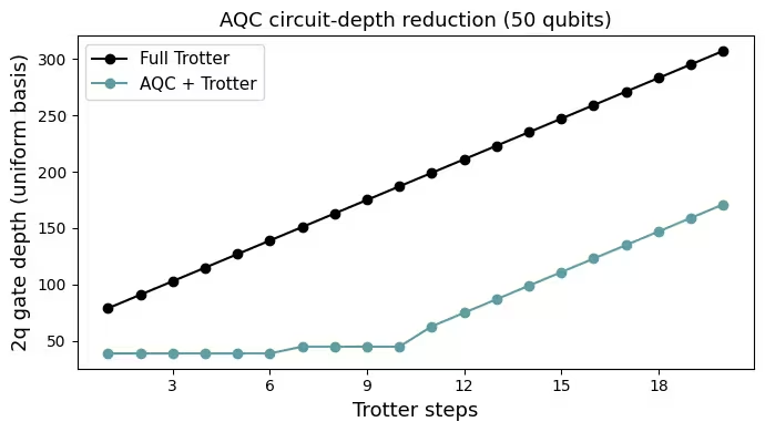
Built 20 circuits, deepest 2q depth (uniform basis) = 307
Defined 50 Z observables.

Step 2b — target MPS:
  k=1: max bond = 44
  k=2: max bond = 46
  k=3: max bond = 53
  k=4: max bond = 62
  k=5: max bond = 75
  k=6: max bond = 96
  k=7: max bond = 118
  k=8: max bond = 128
  k=9: max bond = 128
  k=10: max bond = 128

Step 2c — one-layer ansatz: 2971 parameters, 2q depth (uniform basis) = 39
Step 2c — two-layer ansatz: 3412 parameters, 2q depth (uniform basis) = 45
  k=1: fidelity = 1.0000, 2q depth (uniform basis) = 39, 215.6s
  k=2: fidelity = 0.9676, 2q depth (uniform basis) = 39, 269.8s
  k=3: fidelity = 0.9014, 2q depth (uniform basis) = 39, 293.5s
  k=4: fidelity = 0.8755, 2q depth (uniform basis) = 39, 279.6s
  k=5: fidelity = 0.8450, 2q depth (uniform basis) = 39, 266.4s
  k=6: fidelity = 0.8146, 2q depth (uniform basis) = 39, 371.0s

E0626 02:59:07.229070 1508496 slow_operation_alarm.cc:73] 
********************************
[Compiling module jit_MakeArrayFn for CPU] Very slow compile? If you want to file a bug, run with envvar XLA_FLAGS=--xla_dump_to=/tmp/foo and attach the results.
********************************
E0626 02:59:21.713796 1508477 slow_operation_alarm.cc:140] The operation took 2m14.484932074s

********************************
[Compiling module jit_MakeArrayFn for CPU] Very slow compile? If you want to file a bug, run with envvar XLA_FLAGS=--xla_dump_to=/tmp/foo and attach the results.
********************************

k=7: fidelity = 0.7312, 2q depth (uniform basis) = 45, 10865.3s
  k=8: fidelity = 0.7720, 2q depth (uniform basis) = 45, 1450.3s
  k=9: fidelity = 0.7316, 2q depth (uniform basis) = 45, 3388.6s

E0626 07:21:05.148724 1508496 slow_operation_alarm.cc:73] 
********************************
[Compiling module jit_MakeArrayFn for CPU] Very slow compile? If you want to file a bug, run with envvar XLA_FLAGS=--xla_dump_to=/tmp/foo and attach the results.
********************************
E0626 07:21:24.286095 1508477 slow_operation_alarm.cc:140] The operation took 2m19.137566498s

********************************
[Compiling module jit_MakeArrayFn for CPU] Very slow compile? If you want to file a bug, run with envvar XLA_FLAGS=--xla_dump_to=/tmp/foo and attach the results.
********************************

k=10: fidelity = 0.6726, 2q depth (uniform basis) = 45, 3396.1s

Step 2d — assembled 20 circuits
  At step 20 (uniform basis): Trotter 2q depth = 307, AQC+Trotter 2q depth = 171; 2q gates: Trotter = 3775, AQC+Trotter = 1913

Output of the previous code cell

Backend: ibm_fez
Transpiled 2q depth (deepest, ISA on ibm_fez): 105 (2q gates: 2574)
Job ID: d8v39vhropqc738biotg

Output of the previous code cell

Nire-reproduce ng mga hardware result ang mga pangunahing katangian ng two-spinon continuum: ang scattering intensity ay nakakonsentra malapit sa antiferromagnetic wave vector na $q = \pi$ sa mababang enerhiya at bounded mula sa ibaba ng sinusoidal spinon dispersion, na may malawak na continuum ng spectral weight sa itaas nito sa halip na iisang sharp mode. Ito ang parehong istraktura na nasukat ng inelastic neutron scattering sa KCuF $_3$ , at pinapatunayan nito ang buong workflow ng ground-state preparation, perturbation, AQC-compressed Trotter evolution, at error-mitigated measurement sa sukat na 50-qubit.

Mga susunod na hakbang

Kung interesante para sa iyo ang gawaing ito, maaaring interesado ka sa sumusunod na materyal:

Mga Rekomendasyon

Gayahin ang neutron scattering gamit ang isang AQC + Trotter dynamics Serverless workflow — isang kasamang tutorial na nagpapatakbo ng parehong eksperimentong ito sa pamamagitan ng isang deployed na Qiskit Serverless function template
Lee et al., "Benchmarking quantum simulation with neutron-scattering experiments" (arXiv:2603.15608) — ang reference paper na batayan ng tutorial na ito
Mga error mitigation at suppression techniques — DD, Pauli twirling, at TREX na ginamit sa mga hardware experiment
Approximate quantum compilation para sa time evolution circuits — tutorial sa AQC-Tensor
Dokumentasyon ng AQC-Tensor

Mga learning outcome​

Prerequisites​

Background​

Inelastic neutron scattering at ang dynamical structure factor​

KCuF3_33​: isang canonical na Luttinger-liquid magnet​

Ano ang aming sinisimulate at sinusukat​

Workflow ng quantum simulation​

Approximate quantum compiling (AQC)​

Simulation ng MPS​

Requirements​

Setup​

Halimbawa ng simulator sa maliit na sukat​

Step 1: I-map ang mga classical input sa isang quantum problem​

Step 2: I-optimize ang problema para sa pagpapatakbo sa quantum hardware​

Step 3: Patakbuhin gamit ang Qiskit primitives​

Step 4: I-post-process at ibalik ang resulta sa nais na classical format​

Pagpapatakbo sa malaking sukat na hardware​

Mga susunod na hakbang​

Mga learning outcome

Prerequisites

Background

Inelastic neutron scattering at ang dynamical structure factor

KCuF $_3$ : isang canonical na Luttinger-liquid magnet

Ano ang aming sinisimulate at sinusukat

Workflow ng quantum simulation

Approximate quantum compiling (AQC)

Simulation ng MPS

Requirements

Setup

Halimbawa ng simulator sa maliit na sukat

Step 1: I-map ang mga classical input sa isang quantum problem

Step 2: I-optimize ang problema para sa pagpapatakbo sa quantum hardware

Step 3: Patakbuhin gamit ang Qiskit primitives

Step 4: I-post-process at ibalik ang resulta sa nais na classical format

Pagpapatakbo sa malaking sukat na hardware

Mga susunod na hakbang