Pooled sample-based quantum diagonalization ng isang nuclear Hamiltonian

Tinatayang paggamit: 2.5 minuto sa isang Heron processor (TANDAAN: Isa lamang itong pagtatantya. Maaaring mag-iba ang iyong runtime.)

Hinahanap ang bersyon ng Fortran?

Ipinapakita ng notebook na ito ang implementasyon sa Python. Ang implementasyon sa Fortran ay nasa Fortran companion directory ng repository na ito ng dokumentasyon. Nagdaragdag ang bersyon ng Python ng isang self-consistent na hakbang sa configuration-recovery, na hindi ginagawa ng Fortran driver.

Mga resulta ng pagkatuto

• Alamin kung paano ang isang nuclear shell-model Hamiltonian, na naka-tabula sa isang $J$-coupled basis ng mga orbital, ay nagiging qubit Hamiltonian sa $m$-scheme, kung saan ang isang qubit ay isang single-particle state.

• Bumuo ng isang fixed, non-variational excitation ansatz na ang mga angle ay nagmumula sa second-order perturbation theory, kaya walang classical optimization loop.

• Ihambing ang qubit at fermionic excitation at sukatin kung paano nakakaapekto ang pagpili sa two-qubit depth ng ensemble.

• Patakbuhin ang self-consistent configuration recovery gamit ang qiskit-addon-sqd kapag ang mga napapanatiling dami ay nucleon number, $M_J$, at parity sa halip na electron number at spin.

• Ilapat ang isang workflow mula sa isang 24-qubit na problema na maaari mong suriin nang eksakto hanggang sa isang 40-qubit na problema na may halos dalawang milyong basis state, lampas sa kapasidad ng exact-diagonalization ng tutorial na ito.

Mga paunang kailangan

Bago magsimula, suriin ang mga sumusunod na paksa:

• Sample-based quantum diagonalization at ang SQD addon API reference.

• Sample-based quantum diagonalization of a chemistry Hamiltonian, ang katapat na electronic-structure ng tutorial na ito.

• Transpile against a backend target at Introduction to primitives.

• Second quantization at ang Jordan-Wigner mapping.

Batayan

Ginagamit ng nuclear shell model ang isang nucleus bilang ilang valence na nucleon na gumagalaw sa isang maliit na set ng single-particle orbital sa ibabaw ng isang inert na core, na nag-iinteraksyon sa pamamagitan ng isang empirical two-body force na naaangkop sa sinukat na spectra. Malawakang ginagamit ito sa low-energy nuclear structure. Ang computational cost nito ay combinatorial: ang basis ay bawat paraan ng pamamahagi ng valence protons at neutrons sa mga magagamit na state, at ang paglagong ito ang naglilimita sa mga model space na naaabot ng exact diagonalization.

Hinahati ng Pooled sample-based quantum diagonalization (pooled SQD) [1] ang problemang iyon sa dalawa. Ang isang quantum circuit ay ginagamit lamang upang magmungkahi kung aling mga basis state ang mahalaga. Ito ay sinusukat sa computational basis, at ang bawat nasukat na bitstring ay nagpapangalan sa isang Slater determinant. Ang Hamiltonian ay pagkatapos ay binubuo at dina-diagonalize nang classical sa span ng mga determinant na iyon. Dahil ang classical na hakbang ay isang eksaktong diagonalization sa loob ng isang subspace, nagbabalik ito ng isang variational upper bound sa tunay na ground-state energy, at ang bound ay maaari lamang bumaba habang nadadagdagan ang mga determinant.

Ginagawang noise-tolerant ng paghahating ito ng trabaho ang pamamaraan, na may mahalagang limitasyon. Binabago ng noise kung alin na mga determinant ang minumungkahi ng circuit. Hindi ito pumapasok sa classical Hamiltonian, kaya hindi nito magagalaw ang eigenvalue ng isang partikular na subspace: ang isang shot na lumalabag sa isang napapanatiling dami ay itinatapon o inaayos, at ang isang shot na nakaligtas ay isang lehitimong basis vector kahit paano ito nagawa. Ang noise samakatuwid ay nagkakahalaga sa iyo ng kalidad ng subspace, hindi ng kawastuhan, at ang bilang na iyong iniuulat ay isang upper bound sa magkabilang paraan.

Nagbibigay ang nuclear structure ng ilang eksaktong quantum number para sa pag-filter ng mga sample. Ang isang pisikal na determinant ay dapat magdala ng tamang bilang ng valence protons at ng tamang bilang ng valence neutrons, ang tamang kabuuang angular-momentum projection na $M_J$, at ang tamang parity. Ang bawat isa ay maaaring suriin gamit ang isang integer test sa isang bitstring. Ang bahagi ng mga sample na tinanggihan ay depende sa constraint at model space.

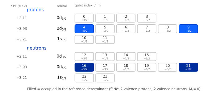
Ang bawat qubit ay isang $m$-scheme single-particle state na $(n, \ell, j, m_j, t_z)$, at ang $|1\rangle$ ay nangangahulugang okupado. Gumagamit ang register ng nakapirming ayos: mga proton muna, pagkatapos ang mga neutron; sa loob ng isang species, mga orbital ayon sa ayos ng file; sa loob ng isang orbital, pababa ang $m_j$. Ang dalawang kalahati ng isang bitstring ay samakatuwid ang proton configuration at ang neutron configuration. Ito ang bipartition na inaasahan ng mga pooled SQD post-processing tool.

Ang workflow

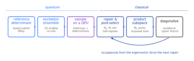
Dalawang yugto sa diagram ang humahawak sa mga nuclear symmetry.

Hinahawakan ng Repair and post-selection ang mga sample na apektado ng hardware noise. Ang dalawang half-register nucleon number ay mga Hamming weight, kaya direktang hinahawakan ito ng qiskit-addon-sqd: inaayos ng recover_configurations ang isang sirang bitstring sa pamamagitan ng pag-flip sa mga bit na pinakahindi tugma sa kasalukuyang pagtatantya ng average orbital occupancy, sa halip na itapon ang shot.

Ipinapakilala ng The product subspace ang $M_J$. Dahil ang $M_J = M_p + M_n$ ay nag-uugnay sa dalawang kalahati, ito ay hindi isang katangian ng alinman sa dalawa, kaya hindi ito dapat gamitin upang i-filter ang buong shot: ang isang bitstring na ang proton half at neutron half ay pareho valid ay nagbibigay pa rin ng dalawang magandang half-configuration kahit na mali ang kabuuang $M_J$ nito. Ang subspace samakatuwid ay saklaw ng bawat produkto ng isang na-sample na proton configuration kasama ang isang na-sample na neutron configuration, kinukuha ang mga produkto na napupunta sa target na $M_J$ at parity sector. Ito ang pooled SQD subspace construction, at ibig sabihin nito ay ilang libong bitstring ay maaaring sumaklaw ng subspace na mas malaki pa sa bilang ng sample.

Dalawang namumunong ekwasyon

Ang shell-model Hamiltonian ay isang one-body term kasama ang isang two-body interaction,

$$\begin{equation} \tag{1} H = \sum_{p} \varepsilon_p\, a_p^\dagger a_p + \tfrac{1}{4}\sum_{pqrs} \langle pq \| rs \rangle\, a_p^\dagger a_q^\dagger a_s a_r , \end{equation}$$

kung saan ang $p,q,r,s$ ay nagla-label sa mga $m$-scheme state at $t_z = -1$ para sa isang proton, $+1$ para sa isang neutron. Ang mga empirical interaction tulad ng USDA [2] at GXPF1 [3] ay naka-tabula hindi sa $m$-scheme kundi sa $J$-coupled basis, bilang mga matrix element na $\langle ab; J | V | cd; J \rangle$ sa pagitan ng normalized antisymmetrized two-body state ng mga orbital na $a,b,c,d$. Ang pagbawi sa $m$-scheme element ay isang Clebsch-Gordan recoupling,

$$\begin{equation} \tag{2} \langle pq \| rs \rangle = \sqrt{1 + \delta_{ab}}\sqrt{1 + \delta_{cd}} \sum_{J} \langle j_p m_p\, j_q m_q | J M \rangle \langle j_r m_r\, j_s m_s | J M \rangle \langle ab; J | V | cd; J \rangle , \end{equation}$$

kung saan binabaliktad ng mga $\sqrt{1+\delta}$ factor ang normalization convention ng mga naka-tabulang state. Ang lahat pang iba sa tutorial na ito ay binuo sa dalawang ekwasyong ito.

Ang tatlong run

	Nucleus	Shell	Qubits	Symmetry-allowed na basis	Eksaktong masusuri?
Maliit ang sukat	$^{20}\mathrm{Ne}$ (2p + 2n)	$sd$	24	640	Oo
Malaki ang sukat	$^{44}\mathrm{Ti}$ (2p + 2n)	$pf$	40	4,000	Oo
Malaki ang sukat	$^{48}\mathrm{Cr}$ (4p + 4n)	$pf$	40	1,963,461	Hindi

Ang small-scale run ang walkthrough. Parehong gumagamit ng 40-qubit register ang dalawang large-scale run: ang una ay maliit pa rin sapat upang i-diagonalize nang eksakto sa isang laptop, kaya maihahambing mo ang resulta ng hardware sa isang eksaktong reference. Ang pangalawa ay lampas sa kapasidad ng exact-diagonalization ng tutorial na ito.

Bawat run dito ay pinapatakbo sa isang QPU. Iyon ay isang pagpipilian na ginawa para sa tutorial na ito sa halip na isang kinakailangan ng pamamaraan: lahat ng tatlong run ay nagbabahagi ng parehong backend at gate budget upang maihambing mo ang kanilang performance sa iba't ibang laki ng problema.

Mga Kinakailangan

I-install ang mga sumusunod na package bago magsimula:

• Qiskit SDK v2.0 o mas bago (pip install qiskit)

• qiskit-ibm-runtime v0.40 or later (pip install qiskit-ibm-runtime)

• SQD addon v0.12 o mas bago (pip install qiskit-addon-sqd)

• NumPy, SciPy, at Matplotlib (pip install numpy scipy matplotlib)

Kakailanganin mo rin ng isang IBM Quantum® account na may mga kredensyal na naka-save nang lokal, at access sa isang QPU na may hindi bababa sa 40 qubit.

Walang kinakailangang simulator package, at walang kailangang i-download na data file. Ang dalawang interaction file na ginagamit ng tutorial na ito ay naka-embed sa sumusunod na setup cell at isinusulat sa isang temporary directory kapag pinapatakbo mo ito.

Pagsasaayos

Ini-import ng seksyong ito ang mga kasangkapan at dine-define ang mga shell-model helper na kailangan ng workflow, sa ayos na ginagamit ito ng workflow. Ang physics sa likod ng bawat isa ay hinango sa Appendix; inilalarawan ng mga comment ang papel ng bawat function sa workflow.

Dalawang interaction file ang unang binubuksan (unpack). Parehong mga nailathalang parameter set, na naka-embed dito upang ang notebook ay self-contained: ang usda.snt ay ang USDA $sd$-shell Hamiltonian [2] at ang gxpf1.snt ay ang GXPF1 $pf$-shell Hamiltonian [3].

# Added by doQumentation — required packages for this notebook
!pip install -q matplotlib numpy qiskit qiskit-addon-sqd qiskit-ibm-runtime scipy

from __future__ import annotations

import base64
import gzip
import itertools
import tempfile
from dataclasses import dataclass
from functools import lru_cache
from math import factorial, sqrt
from pathlib import Path

import matplotlib.pyplot as plt
import numpy as np

from qiskit import QuantumCircuit
from qiskit.circuit.library import PauliEvolutionGate
from qiskit.quantum_info import Operator, SparsePauliOp
from qiskit.transpiler.preset_passmanagers import generate_preset_pass_manager
from qiskit_addon_sqd.configuration_recovery import recover_configurations
from qiskit_addon_sqd.counts import bit_array_to_arrays
from qiskit_addon_sqd.subsampling import postselect_by_hamming_right_and_left
from qiskit_ibm_runtime import QiskitRuntimeService, SamplerV2

from scipy.linalg import eigh

_USDA_SNT_GZ = (
    "H4sIAI5wqWoC/4WY224bRwyG7/UU9F0CONsZco5AUyBuC/QmQNG06KWhWGql1LYMy+kJefiOTrucGXJrQAgsf5nl8ecOr+CX"
    "D9+9g/0K9pv1/T389rx7gPLrsH+Cz/vVctg+vgAsrgB+HeDdAD9t7zYv6+dr+DDA+z8223/X17B8XMFN+ev9+m+4ed799XjA"
    "f9z8sy/4+s8BvoWYrsEERwbhFRqTXi+uCvOwW63vYf+0vFvDAgDo/AFIh8/hK7DH30354Omvb8o3V8c/vIUnMKtboK/wiGKF"
    "+gnFEfVn9PQUe8bthNIRtftbsGfUtQbAGXUFfawM8K0BF9SP6MWA0BpwQcMRvRhwBSX86+fl3ct2d4jq4+eHa3hYv2x2q7fX"
    "AJuPy+fb3cP69+Uh4luAT8djv95++eGV/fj6y6dvFudnmcX4lGOoBmttNOVncTL2FLs3NGT0l++ndJTv0cR8/t6NUanP8WMI"
    "6nPC6C8/5wp+vnn//QLOP9ank3k2wRszkDn/Zwv15xiv41l2SDmjhuEFM4PJ0QkYcgzM4A1Jp1GDkcvtaWMAR9tosAa9huHk"
    "AtoUBYwaF8hGarAxOywgxnoeN+Se2smF4H3QMPZQ653XMJpOi6GyrcLcZJtzLgoYcdsOyXKibV1Aom0fikJO0VLUMDeW3kAl"
    "qQLWpd66qGE02eZ9lXqSPD3UWyl5DeOeGnINJnmaUggCVrtgh2DJNm3fVy8WF3LSMFa9hYga5iYX0IQsYK2nmTpJkoq81Acy"
    "jLTTnPEaxqo3JGcbvZMeGnJVbw6mf2cUqcIsO80nFdOFq8JoSlY+Zb7FfNNZlnw2PqOE8SL3PtlSJhJGXGqsDRjbh4bmocWy"
    "oiIxSxjv09JYgaxlGLZxA9EFFOImuIBt3EB04TK3Z5S8wizrrFCJQ4Xpgl9hzDYbu0LCNm6HzkJHweUkYazITalyF7NjGAnh"
    "FZJFQniFZFHnqWgbdZ6qtoX50VZhvEJ81TJe7AUcQozH8yQMJ8ymUS07jLin6LXT3FRIhmwSTmtbJpEjr2AsvM7E1ra+ZaiM"
    "NoxewZinBlPQTmPJyikn7TQ2630SbWuz4CLlwzuGhCHPqbUmRZQwpkiBDn1vsoQ55oKjbEvNNVgbXls0WvA0NKnPpku91Fkx"
    "pahhXPDJtxVCQkBcMtJD27I8VJGAhWYYlVuZzc5e+jSIZWnLa57nOQ1iWZY+jSE3GP5/QIKi5E1Agqi9BbMZiUjEWNwChqKq"
    "KTZY11ku5ca2Pqc4YKk1o2DstBjJC1htW2nAgEZ4aDdPvQmmmLeY4tWFt9Y3VAdlpW+oDcpa3zpM1jdUB2XV9agOyqrrcWZQ"
    "sq7vMMffBseux5l5yjoLZ+Yp6yzU5mmt5DgzT5mSozZPoVIknJmnTJFQHZRV12OrlvpFQFbycoGKOWiYfl9QlXySGtSUvL9W"
    "VJi/YG4grC4CmuCX6CZrKUsY64UyJolCQoZJqWeKhDOCzxQJNcGXbZMEX7EtzF+gvCI1npxjmKaW5Q06ewVjOY0u2+Y0kt5D"
    "JhlETS2P+5CqyIMYkCI1NK50SO3TarSR2qfVaKOZPmXjg2beVJmS01zqp/CSmvoqvNSOD/kaS+qUoSGaTM2yz83fdjtMvsZy"
    "xOv7N44Fff/GT5q5tXWYfB3jWND3b9yumUvK5SQnvK6w/VuHyfu3DpP3bx0m7984FvT9W4fJ+zceWq/v3zpM3r9xLOj7tw6T"
    "928X053QgGz/1mHy/u3yZ8lTtn/jWND3b74NiDx2vRbeep56Lbz1oPRaeOv9G0dmxofXPK33bx0m798C1B9RuP4DPJ0WcLAa"
    "AAA="
)

_GXPF1_SNT_GZ = (
    "H4sIAI5wqWoC/4WcQY8dtw3H7/kU41sCeF8lUqKkQw9NgbaXoEHQQ26BkdiIEWdt2E6L9tNXb9+ORIn8PwdZILB/S3I4IsW/"
    "ZiYvjr//+P3f4nG8ef/x+PDm4dOvr9+9++rF8d3l+Mf7x99fvTz+dTn++fnTH7/1//z28pfL8e3H9/95fHm8evzl+lffvf3f"
    "H59e/fb26L9zHN//+t9Pl+OH1/++HH89JL88gkQO8esfvjm+phDomyvW//39/S+v3x2fPrz6+fVX/dfS889B4fpz/aN43P7p"
    "f3Bw/ynH8fD0Zy+uf/fn48MR3vxU/kRXlp7Z+PzDiqUnNn74iW8sb3azYvm0m29s2uxGxabTbryx2cZ7nGzu7KOKV2y8g5Un"
    "dsZbbLyDLafd53irjXew9bR7jffF8fbx8+uPr37+/Pb941dPv3P93ZH4W/If6kUohXCm+Jbmh3yR0jicybwl9CFeuFILy908"
    "HtIlcrlZyCNJ2q6MdGi7ZVy4tlvHJS52Y71FnHp8D+HCIYTlQuYFhdsv0yVxzZB6vsxwaZwJUumkIjWB1POdDhcqlR2KVo85"
    "SoDU8NgdNodiZevqMUqB1LCVWsO2ZMQlyYs+bXEFk4m5bMJJlVgSpGjaouhQvFKxUIbUjIvI85hWW4FNvubyDnMxMkFKRc8V"
    "Uml65OhQW1x9fe3XOAtsZPXJ36TIX18SaoQUnysnZsHUXPfcKqTyaSu36FHbWg0tN0jxWIXEAVLzbqcqkMpj3T8lwlBp9RhD"
    "qpAaHpnzni9nRXPh6lDbysmJBVLzDtU71KztnDxqW1+JhDaKnTtUa4DUzH00Hp0VXQMHSM3c16irlpf7GEcN1dogpfpEDpAa"
    "WRUOBKl0UqkIQ2qs+5IYU6OvthbFodIaF6/9i51VeF0TLZSN2lfh9T729utQOqtXKi/dl/21mihhW+M+BpIKqblypDWHSntc"
    "mSA1O3nMe+6dHp0DEaRmXCU0h9p7dOYCqVm1MehOnvy7nWphSKnuu+Q++X2Ca4uQGrYkxp3yMkFLL0ygavPovmR64dhFY5QM"
    "KVK1XRxqX4UydlHCXU44hY1ydndKuUBK11BzqH1NNOKNMvt27PMXVUWBemSqCVIjrr4nYFtzTSQJkJp3O7se09p9YygCKVL7"
    "UN4opx5DNnE5q5AlerZ2jyExpEYmggTtMYFrzC1Bak58jetGeSvHenSip9ROik0m5lqdsxzjrCYhTM1uImOHYZzVPvnWjXIm"
    "0RoaKyqhjjlqiEE3uWoYHqopbT/KY0pDD+Xtx9d8lvI0n6U8zWcpT/NpQqDms5Sn+TRVoOazlKf5LOVpPk1VqPl05AI1n6U8"
    "zaepAjWfpTzNp6kKNZ/OQoGaz1Ke5rOUp/k0VaHm03mvUPOd1+esL6X5LOVpPkt5ms9SnubTVIGaz1Ke5rOUp/ks5Wk+TVWo"
    "+SzlaT69mgVqPk0VqPks5Wk+S3maT1MVaj5dPwVqPkt5mk9TFWo+S3ma77x/8z56ms9SnuazlKf5LOVpPkt5ms9SnubTVIWa"
    "z1Ke5jupfRWumk9TBWo+S3maz1Ke5rOUp/k0VaHms5Sn+XTnLVDzWcrTfJqqUPNZytN85/1z7rbSfJbyNN/5t06fUJrPUp7m"
    "OykvE7T0wgqqdmo+Mb3Q03yCO6bSfII7ptJ8gruc0nxi+pen+eROL5yaT3CXU5pPx1Sh5hNcj0rzCajHVfMJqMdV88mdesyu"
    "xwo1n+B6VJpPcD0qzSe4HpXmE1yPSvMJrkelwERVR4Waz1Ke5hNTQ3THoxO90nzFZMLTfAVnVWm+grOqNF/BWVWaTxMVar6C"
    "r1FpvgK6yar56vbja76onormu8/5ViqOrNblZH6l0NPAlRq9sKaIbaFnhis15tUuH/E1oieLK1XOTIgsz3ROap9XpQ/SJWqK"
    "bCYcKm6K4tp9iUqqzbd1j4qO+g2tpTV6sll1qLipk6fnw32/isDWPSruPborwz7x9eakKbbry6Gi7RN9nrhuHr4tPXXsVLT9"
    "vvTdKlUQ18i9Q0Wn+2ZOlYpva0yiDhXthNz69p4S+7ZG7h0q2jma+/BIIfm2RnU4VLQ9R6hG4iWryVurhorOlNbzEJr4tubk"
    "bim6e25iqbFbJY4MKfREfaXGNXKK2aF2BSapD6Oy5162yd1S5Og0iq3k5tua1WEpsus+ZO4ZS76tqU4sRc7+mAtJyL6teR8t"
    "RVbDUO9yXM2a2O6jQ5GjdCi3HKpva04dluK7J1uWGtFLjhFS6J2HlZpKhzOm0JsRK5XnmjD7Izv5av0eBd7zVb5IsVU6ffTN"
    "oQXf1peoeveNjZWaNURFZ0L8fTsX1s9hwO4eeHkOA3Z3Zct6ZOccgPAM0O91hR4ZPEcWMAPkdBWQvsdZj72xZuTRs2U95qFY"
    "a8FZHVQpy/Mhd55YbGmPew2VGB2PRvOVsNlib0orYbO1U8fi0cbF6uQhw7jUycMybYs/dSiKwGxyLB5tXEmdM5WM4lKnGLFm"
    "FFeaPTruK8ehlEcbV55n2yIwrnlOXorAuPKsxyIwrjz7l3greptzSgve+tqo2lLbcu9MQ4oiPDMpjzaueR8rUUZxqaql/T46"
    "k5WiCM9fyuNpy5uZpM9WkvfaxpS1Ndd96JKV2LflUdrW1idaKOT0HNMnTCdnT/OZvcOZv5RHG5fqAJFhXLO2WykwrtlzJkV4"
    "llMebVxp7kOUMopr7h1dSmcUl9LuxesT2z6kPOq4ttkkk7sj1/1JWWWnHvfdfVKE50LlUV+jObPqs2hO+zViytpSJ+CFSyu+"
    "LY+yttRM3gf3HH1bHmVtzR5NXZQXcI0epW1tdyh2d86a2O52F9vR6V8FUgTm1dWjjWuepZUgMK45k2cKMC6PIjD7rh6j+gpi"
    "0Y904b675/n2h3u6QteTedkoc7qy2LIeaUxpkXNAHgeV53khozOYxZb1qDpTrvAa+TxBClECvEbPlvWY5o4cA7zGNDSfFIbX"
    "6NmyHmd1SEnwGgfVJ6YKr9GzZT3KebdDZIYe5bzGQLFAj54t7XHXfDkmJ6v789r17e7iTEMrxXhmUh5tXHNmainCuObMVBOO"
    "y6MYzEyrx9MW2VMf4cC9NWlbzpmVoqytucPkIO12SsZ4/lKUtTX7V6LGsfi2phadlLa1nX89naUHc437uYnQni/nlEzWN/S8"
    "s7TVo41LvUsW9+pwqFBl79HsPYkVr/sK9GjjYnVWSzBfqjoowXx5FN+ZC6dHG5d6WybjfM15ouYE8+VRDObC1aOOa3v+WEJq"
    "Tlzb2VCRELOtbYEU47NH5dHGpd5nagzj0s+HAozLoxjMq6tHnfutHmNjblz23G/1qChra3rMOT6f3jGefRVlbamZKfR1COKa"
    "PWdS1tZcXy3mnMm3pd4IGpS1Nd9Uai0Wir6t+fxxUtrWPvu27M1MG8XJ1KMz+yqK8Vmt8mjjmn1CKmcUF88zhVIzimtOtZNi"
    "fO6rPGpbW9XGLrg50G5rfwNhUueu7swmEtI55yQ0m/RpqI3JPd15ujVtWY9TSbcxpSU8dSShAj16tk4b3r6dmUlI2/L27Ulp"
    "W7vKLFK3uByK4nI2VP19SFEJ7EOrRxvXyESr413YhPchLsssV/0dRlEJ70PKo7a1n/vWa1rLbsu8mTooa0up8tpyEd+Wep42"
    "KG1rf6su5ebkvpqztLzl3qltRSVc28ojmTM+9F2TwNm3Qgp9/eSeKnaNXFtwqH3nk1KaJE05M6ZDOdNjv9NJIvm2Zr+3lFeP"
    "EvqGnH1bM/eWMtNQvFCRHnzUlJlzXMqZYFKqHHLxbdFUFIbiu+8XWmo+50vL6R06l1u/PBO/asN8B5zAmdXTDtP7r8h+jeWL"
    "lFOPocYumti39SWq3v0iTvxdtDw9hhmUq9N6PbaqvzJyqyNeMi0nIm51LLbojgIrOUKP+l2yBj16tghrqxib1gqg0pLknfIq"
    "bdoirJqkMMNrnDNATPgaPVuE9VBv0J7HbU107V42W44eUhSjPrF4JKyHUokZxqXeTV+exAI9pCjGp/zKIwE9dO2+XSTX1vbc"
    "b6pJUYT1UOCWWw2+rdmZJkVYD1Ef0Uoi39acySdFWA9RztLVjm9LPQ0cFAENc3unJjrVsWuY0mK297EYxbrbcs7vlUfCGib3"
    "bQ/GNWffMijCGkZRDHr0w+KRsIbpnem6dnZbe9VOitTsW7e3I+e7Pgnv7tfHQxvl7O7KlvU4zu95fouUUNV21RSGFk2oHhdb"
    "ZGbf+b4cXf8nRlnb8maASVlbc+UkSnSb0hKox4eFIjNHz7c/aHydkvC6T9Lydo3Je+u8ZSdf+xsu06O2ta2vPr70W1l2W9v6"
    "UhSbPoG+kwYnSDVnTKGvqYvfv3JuDVLom2vvpOZpvh9fizHuX71jVp79vqDcG8rrJolLnecTxe8TgMLfBTDoJteOGUVntYJr"
    "5PHOVsKnUaEuJw8oE9MWA5V5e2tA9wmQrw5xQB6RrernS33VkEB1PCmKW5f7P6zudeW7TwAA"
)

DATA = Path(tempfile.mkdtemp(prefix="nuclear_sqd_"))
for name, blob in (("usda.snt", _USDA_SNT_GZ), ("gxpf1.snt", _GXPF1_SNT_GZ)):
    (DATA / name).write_bytes(gzip.decompress(base64.b64decode(blob)))

    if not (DATA / name).is_file():
        raise RuntimeError(f"{name} did not unpack to {DATA}")

Ang model space at ang qubit register

Hawak ng isang .snt file ang model space, ang single-particle energies, at ang $J$-coupled two-body matrix elements. Para sa mga mass-dependent na interaction na ginamit dito, ang ikatlo at ikaapat na field ng two-body header ay tumutukoy sa reference mass $A_{\mathrm{ref}}$ kung saan na-fit ang interaction at ang exponent ng mass dependence nito. Parehong file ay may exponent na $-0.3$, kasama ang $A_{\mathrm{ref}} = 18$ para sa USDA at $42$ para sa GXPF1, kaya dapat i-rescale ang mga naka-tabulang matrix element sa pamamagitan ng $(A/A_{\mathrm{ref}})^{-0.3}$ para sa nucleus na kinukwenta [2], [3]. Hindi kinukumpuni ang single-particle energies. Ang pagligtaan sa hakbang na ito ay nagbabago sa correlation energy ng ilang porsyento.

Ang mga energy na sumusunod ay mga valence na energy, na sinusukat mula sa inert core; hindi ito mga eksperimental separation energy.

@dataclass(frozen=True)
class Orbital:
    idx: int
    n: int
    ell: int
    j2: int
    tz: int  # j2 = 2j; tz = -1 proton, +1 neutron

@dataclass(frozen=True)
class SPState:
    """One m-scheme single-particle state, i.e. one qubit."""

    orb: int
    j2: int
    mj2: int
    tz: int
    ell: int
    spe: float  # mj2 = 2 * m_j

@dataclass
class ModelSpace:
    orbitals: list
    spes: dict
    tbmes: dict
    core_z: int
    core_n: int
    mass_number: int
    a_ref: int
    mass_exponent: float
    mass_factor: float

def read_snt(path, n_protons, n_neutrons):
    """Parse a .snt interaction file, applying its mass dependence for this nucleus.

    The two-body header line is ``n_tbme  method  A_ref  exponent``.  When ``method`` is 1 the
    tabulated matrix elements are rescaled by ``(A / A_ref) ** exponent``, where A is the mass
    number of the whole nucleus -- the core plus the valence nucleons.  A is derived from the
    file's own core numbers rather than passed in, so it cannot silently disagree with the
    valence counts the rest of the workflow uses.  Single-particle energies are not rescaled.
    """
    rows = [
        ln.split("!")[0].split() for ln in Path(path).read_text().splitlines()
    ]
    rows = iter([r for r in rows if r])

    n_p_orb, n_n_orb, core_z, core_n = (int(x) for x in next(rows)[:4])
    orbitals = [
        Orbital(*(int(x) for x in next(rows)[:5]))
        for _ in range(n_p_orb + n_n_orb)
    ]

    spes = {}
    for _ in range(int(next(rows)[0])):  # "i  i  <i|H(1b)|i>"
        field = next(rows)
        spes[int(field[0])] = float(field[2])

    n_tbme, method, a_ref, exponent = next(rows)[:4]
    n_tbme, method, a_ref, exponent = (
        int(n_tbme),
        int(method),
        int(a_ref),
        float(exponent),
    )
    mass_number = core_z + core_n + n_protons + n_neutrons
    factor = (mass_number / a_ref) ** exponent if method == 1 else 1.0

    tbmes = {}
    for _ in range(n_tbme):  # "a  b  c  d  J  value"
        field = next(rows)
        tbmes[tuple(int(x) for x in field[:5])] = float(field[5]) * factor

    return ModelSpace(
        orbitals,
        spes,
        tbmes,
        core_z,
        core_n,
        mass_number,
        a_ref,
        exponent,
        factor,
    )

def m_scheme_states(ms):
    """The qubit register: protons then neutrons, orbitals in file order, m_j descending."""
    return [
        SPState(o.idx, o.j2, m2, o.tz, o.ell, ms.spes[o.idx])
        for tz in (-1, +1)
        for o in ms.orbitals
        if o.tz == tz
        for m2 in range(o.j2, -o.j2 - 1, -2)
    ]

Clebsch-Gordan recoupling

Nangangailangan ang Equation (2) ng mga Clebsch-Gordan coefficient para sa half-integer na angular momenta. Ang bawat argument ay ipinapasa bilang dalawang beses ang pisikal na halaga nito, kaya ang $j = 5/2$ ay pumapasok bilang 5 at nananatiling eksakto ang arithmetic.

Hinahawakan ng Interaction.v_ms ang mga lookup ng interaction matrix element. Iniimbak ng isang .snt file ang bawat matrix element nang isang beses lamang, kaya maaaring kailanganin ng lookup ang antisymmetrized pair-exchange phase na $-(-1)^{j_a + j_b - J}$ sa alinmang panig, at maaaring naka-imbak ang bra at ket sa alinmang ayos.

@lru_cache(maxsize=None)
def clebsch_gordan(j1_2, j2_2, J_2, m1_2, m2_2, M_2):
    """<j1 m1 j2 m2 | J M>.  Every argument is twice its physical value."""
    if m1_2 + m2_2 != M_2 or not abs(j1_2 - j2_2) <= J_2 <= j1_2 + j2_2:
        return 0.0
    if abs(m1_2) > j1_2 or abs(m2_2) > j2_2 or abs(M_2) > J_2:
        return 0.0
    if (j1_2 + j2_2 - J_2) % 2 or (j1_2 - m1_2) % 2 or (j2_2 - m2_2) % 2:
        return 0.0

    f, half = factorial, lambda x: x // 2
    prefactor = sqrt(
        (J_2 + 1)
        * f(half(j1_2 + j2_2 - J_2))
        * f(half(j1_2 - j2_2 + J_2))
        * f(half(-j1_2 + j2_2 + J_2))
        / f(half(j1_2 + j2_2 + J_2) + 1)
        * f(half(J_2 + M_2))
        * f(half(J_2 - M_2))
        * f(half(j1_2 - m1_2))
        * f(half(j1_2 + m1_2))
        * f(half(j2_2 - m2_2))
        * f(half(j2_2 + m2_2))
    )
    total = 0.0
    for k in range(half(j1_2 + j2_2 - J_2) + 1):
        d = [
            half(j1_2 + j2_2 - J_2) - k,
            half(j1_2 - m1_2) - k,
            half(j2_2 + m2_2) - k,
            half(J_2 - j2_2 + m1_2) + k,
            half(J_2 - j1_2 - m2_2) + k,
        ]
        if all(x >= 0 for x in d):
            total += (-1) ** k / (
                f(k) * f(d[0]) * f(d[1]) * f(d[2]) * f(d[3]) * f(d[4])
            )
    return prefactor * total

class Interaction:
    """Antisymmetrized m-scheme two-body matrix elements <pq||rs>, per Eq. (2)."""

    def __init__(self, model_space, sp):
        self.ms, self.sp, self._cache = model_space, sp, {}

    def _tbme(self, oa, ob, oc, od, J, j_ab_2, j_cd_2):
        """<oa ob; J|V|oc od; J>, allowing for how the file happens to order each pair."""
        table = self.ms.tbmes
        # |ba; J> = -(-1)^(j_a + j_b - J) |ab; J> for a normalized antisymmetrized pair;
        # dropping the leading minus makes v_ms symmetric instead of antisymmetric, and
        # the Hamiltonian then fails the rotational-invariance check in Step 1.
        phase_ab = -1.0 if (j_ab_2 // 2 - J) % 2 == 0 else 1.0
        phase_cd = -1.0 if (j_cd_2 // 2 - J) % 2 == 0 else 1.0
        for keys, phase in (
            (((oa, ob, oc, od), (oc, od, oa, ob)), 1.0),
            (((ob, oa, oc, od), (oc, od, ob, oa)), phase_ab),
            (((oa, ob, od, oc), (od, oc, oa, ob)), phase_cd),
            (((ob, oa, od, oc), (od, oc, ob, oa)), phase_ab * phase_cd),
        ):
            for key in keys:
                value = table.get(key + (J,))
                if value is not None:
                    return value * phase
        return 0.0

    def v_ms(self, p, q, r, s):
        """<pq||rs>, zero unless M_J and charge are conserved."""
        cached = self._cache.get((p, q, r, s))
        if cached is not None:
            return cached

        P, Q, R, S = (self.sp[i] for i in (p, q, r, s))
        value = 0.0
        if P.mj2 + Q.mj2 == R.mj2 + S.mj2 and P.tz + Q.tz == R.tz + S.tz:
            M = P.mj2 + Q.mj2
            # sqrt(1 + delta): undo the normalization of the tabulated pair states
            c12 = sqrt(2.0) if (P.tz == Q.tz and P.orb == Q.orb) else 1.0
            c34 = sqrt(2.0) if (R.tz == S.tz and R.orb == S.orb) else 1.0
            for J2 in range(
                max(abs(P.j2 - Q.j2), abs(R.j2 - S.j2)),
                min(P.j2 + Q.j2, R.j2 + S.j2) + 1,
                2,
            ):
                cg_bra = clebsch_gordan(P.j2, Q.j2, J2, P.mj2, Q.mj2, M)
                cg_ket = clebsch_gordan(R.j2, S.j2, J2, R.mj2, S.mj2, M)
                if abs(cg_bra) < 1e-12 or abs(cg_ket) < 1e-12:
                    continue
                value += (
                    c12
                    * c34
                    * cg_bra
                    * cg_ket
                    * self._tbme(
                        P.orb,
                        Q.orb,
                        R.orb,
                        S.orb,
                        J2 // 2,
                        P.j2 + Q.j2,
                        R.j2 + S.j2,
                    )
                )

        self._cache[(p, q, r, s)] = value
        return value

Matrix element at ang symmetry test

Ang isang determinant ay isang pinagsunod-sunod na tuple ng mga okupadong qubit index. Ang dalawang determinant na naiiba sa higit sa dalawang okupadong state ay may nawawalang matrix element; kung hindi, ang mga Slater-Condon rule ay nagbibigay ng maikling sum sa interaction, na pinarami ng isang fermionic sign na bumibilang kung ilang okupadong state ang nasa pagitan ng mga operator sa nakapirming ayos ng register.

Ang symmetry_allowed ay ang integer test na kinabubuuan ng lahat ng apat na eksaktong quantum number. Ginagamit ito parehong upang i-filter ang mga sample at upang i-enumerate ang eksaktong basis para sa mga run na sapat kaliit upang suriin.

def matrix_element(inter, det_a, det_b):
    """<A|H|B> for two determinants, each a sorted tuple of occupied qubit indices."""
    set_a, set_b = set(det_a), set(det_b)
    out_a, out_b = sorted(set_a - set_b), sorted(set_b - set_a)
    if len(out_a) != len(out_b) or len(out_a) > 2:
        return 0.0

    if not out_a:  # diagonal: one-body plus two-body
        return sum(inter.sp[i].spe for i in det_a) + sum(
            inter.v_ms(i, j, i, j)
            for i, j in itertools.combinations(det_a, 2)
        )

    if len(out_a) == 1:  # one state moves, p -> q
        p, q = out_a[0], out_b[0]
        crossings = sum(1 for k in set_a if min(p, q) < k < max(p, q))
        return (-1.0) ** crossings * sum(
            inter.v_ms(p, j, q, j) for j in det_a if j not in (p, q)
        )

    (p, r), (q, s) = out_a, out_b  # two states move
    crossings = sum(1 for k in set_a if p < k < r) + sum(
        1 for k in set_b if q < k < s
    )
    return (-1.0) ** crossings * inter.v_ms(p, r, q, s)

def subspace_hamiltonian(inter, dets):
    """Dense real-symmetric H projected onto the span of `dets`."""
    H = np.zeros((len(dets), len(dets)))
    for a, det_a in enumerate(dets):
        H[a, a] = matrix_element(inter, det_a, det_a)
        for b in range(a + 1, len(dets)):
            H[a, b] = H[b, a] = matrix_element(inter, det_a, dets[b])
    return H

def ground_state(inter, dets):
    """Lowest eigenvalue and eigenvector of H over `dets`."""
    values, vectors = np.linalg.eigh(subspace_hamiltonian(inter, dets))
    return values[0], vectors[:, 0]

def symmetry_allowed(
    sp, det, n_protons, n_neutrons, mj2_target=0, parity_target=0
):
    """The four exact shell-model quantum numbers, as integer tests on one determinant."""
    n_p = sum(1 for i in det if sp[i].tz == -1)
    return (
        n_p == n_protons
        and len(det) - n_p == n_neutrons
        and sum(sp[i].mj2 for i in det) == mj2_target
        and sum(sp[i].ell for i in det) % 2 == parity_target
    )

def full_basis(sp, n_protons, n_neutrons, **targets):
    """Every symmetry-allowed determinant.  Only tractable for small model spaces."""
    protons = [i for i, s in enumerate(sp) if s.tz == -1]
    neutrons = [i for i, s in enumerate(sp) if s.tz == +1]
    return [
        p + n
        for p in itertools.combinations(protons, n_protons)
        for n in itertools.combinations(neutrons, n_neutrons)
        if symmetry_allowed(sp, p + n, n_protons, n_neutrons, **targets)
    ]

def count_basis(sp, n_protons, n_neutrons, mj2_target=0, parity_target=0):
    """How many determinants `full_basis` would return, without enumerating them.

    A dynamic program over (occupied count, sum of 2*m_j, parity) per species.  This stays
    cheap when the basis itself is far too large to build, which is how the largest run below
    can report the size of the space it is sampling from.
    """

    def species(states, k):
        table = {(0, 0, 0): 1}
        for s in states:
            for key, value in list(table.items()):
                count, m_sum, parity = key
                if count < k:
                    nxt = (count + 1, m_sum + s.mj2, (parity + s.ell) % 2)
                    table[nxt] = table.get(nxt, 0) + value
        totals = {}
        for (count, m_sum, parity), value in table.items():
            if count == k:
                totals[(m_sum, parity)] = (
                    totals.get((m_sum, parity), 0) + value
                )
        return totals

    left = species([s for s in sp if s.tz == -1], n_protons)
    right = species([s for s in sp if s.tz == +1], n_neutrons)
    return sum(
        a * b
        for (mp, pp), a in left.items()
        for (mn, pn), b in right.items()
        if mp + mn == mj2_target and (pp + pn) % 2 == parity_target
    )

Ang reference determinant

Ang ansatz ay binuo sa ibabaw ng isang solong determinant, kaya dapat na ang determinant na iyon ang pinakamahusay na mayroon. Ang pagpuno sa mga pinakamababang single-particle energy ay hindi isinasaalang-alang ang two-body interaction. Sa mga model space na ito, ang pagpiling iyon ay nagbibigay ng energy na 1–2 MeV sa itaas ng determinant na may pinakamababang energy.

Ang paglilimita sa mga filling na binubuo ng time-reversed na $(+m_j, -m_j)$ na mga pares ay pumipilit sa $M_J = 0$ nang eksakto at iniiwan lamang ang $\binom{n_{\mathrm{pairs}}}{k}$ na kandidato bawat species (ilang libo lang ang pinakamarami), kaya ang pinakamahusay ay matatagpuan sa pamamagitan ng paghahanap sa lahat ng ito sa buong diagonal na $\langle \Phi | H | \Phi \rangle$. Ang mga tie ay napupunta sa mga pares na pinakamalakas na naka-align, kung saan pinakamalakas ang $J = 0$ pairing force. Sa bawat kaso sa tutorial na ito na maaaring suriin laban sa isang buong enumeration, ibinabalik ng paghahanap ang global na determinant na may pinakamababang diagonal, na siya ring pinakamalaking solong bahagi ng eksaktong ground state.

def reference_determinant(sp, inter, n_protons, n_neutrons):
    """Lowest-diagonal determinant built from time-reversed (+m_j, -m_j) orbital pairs."""
    if n_protons % 2 or n_neutrons % 2:
        raise ValueError(
            "an odd valence count has no time-reversed paired reference at M_J = 0"
        )

    def species_pairs(tz):
        return [
            (
                q,
                next(
                    p
                    for p, t in enumerate(sp)
                    if t.tz == tz and t.orb == s.orb and t.mj2 == -s.mj2
                ),
            )
            for q, s in enumerate(sp)
            if s.tz == tz and s.mj2 > 0
        ]

    best = None
    for chosen_p in itertools.combinations(species_pairs(-1), n_protons // 2):
        protons = tuple(q for pair in chosen_p for q in pair)
        for chosen_n in itertools.combinations(
            species_pairs(+1), n_neutrons // 2
        ):
            det = tuple(
                sorted(protons + tuple(q for pair in chosen_n for q in pair))
            )
            # break ties toward the most aligned pairs, where J = 0 pairing is strongest
            score = (
                matrix_element(inter, det, det),
                -sum(abs(sp[q].mj2) for q in det),
            )
            if best is None or score < best[0]:
                best = (score, det)
    return best[1]

Ang excitation pool at ang perturbative ranking nito

Dinadala ang correlation ng two-particle–two-hole ($2p2h$) na excitation mula sa reference. Dalawang selection rule ang nagpapaliit sa pool bago mabuo ang anumang circuit: ang isang excitation ay dapat mag-conserve ng $M_J$, at ang hole pair at particle pair ay dapat makapag-couple sa isang karaniwang kabuuang $J$, na isang triangle inequality.

Ang natitirang mga excitation ay inaayos ayon sa Epstein-Nesbet second-order score ng selected configuration interaction [4],

$$\begin{equation} \tag{3} s_\alpha = \frac{|\langle \Phi_{\mathrm{ref}} | H | \alpha \rangle|^2}{|\Delta_\alpha|}, \qquad \Delta_\alpha = H_{\mathrm{ref},\mathrm{ref}} - H_{\alpha\alpha}, \end{equation}$$

na nagtatantya kung gaano karaming correlation energy ang dala ng bawat excitation. Ang parehong dalawang numero ang nagtatakda ng circuit angle: gamit ang $V = \langle \Phi_{\mathrm{ref}} | H | \alpha \rangle$, ang first-order amplitude ay $t_\alpha = V / \Delta_\alpha$. Ipinapaliwanag ng Appendix kung bakit ang first-order amplitude ang pinili sa tutorial na ito sa halip na ang eksaktong two-level angle.

def excitation_pool(sp, occ):
    """2p2h quadruples (h1, h2, v1, v2): same-species pairs, then proton-neutron pairs."""
    holes = {tz: [i for i in occ if sp[i].tz == tz] for tz in (-1, +1)}
    virtuals = {
        tz: [i for i, s in enumerate(sp) if s.tz == tz and i not in occ]
        for tz in (-1, +1)
    }
    pool = [
        (h1, h2, v1, v2)
        for tz in (-1, +1)
        for h1, h2 in itertools.combinations(holes[tz], 2)
        for v1, v2 in itertools.combinations(virtuals[tz], 2)
    ]
    pool += [
        (h1, h2, v1, v2)
        for h1 in holes[-1]
        for h2 in holes[+1]
        for v1 in virtuals[-1]
        for v2 in virtuals[+1]
    ]
    return pool

def conserves_symmetry(sp, op):
    """Keeps M_J, and the hole and particle pairs share a reachable total J."""
    h1, h2, v1, v2 = op
    if sp[v1].mj2 + sp[v2].mj2 != sp[h1].mj2 + sp[h2].mj2:
        return False
    return max(abs(sp[v1].j2 - sp[v2].j2), abs(sp[h1].j2 - sp[h2].j2)) <= min(
        sp[v1].j2 + sp[v2].j2, sp[h1].j2 + sp[h2].j2
    )

def en_denominator(inter, occ, holes, virtuals, floor=0.1):
    """Epstein-Nesbet gap: bare gap, spectator rearrangement, and the pair's own term."""
    gap = sum(inter.sp[h].spe for h in holes) - sum(
        inter.sp[v].spe for v in virtuals
    )
    for k in occ:
        if k in holes:
            continue
        gap += sum(inter.v_ms(h, k, h, k) for h in holes)
        gap -= sum(inter.v_ms(v, k, v, k) for v in virtuals)
    gap += inter.v_ms(holes[0], holes[1], holes[0], holes[1])
    gap -= inter.v_ms(virtuals[0], virtuals[1], virtuals[0], virtuals[1])
    return gap if abs(gap) >= floor else (floor if gap >= 0 else -floor)

def rank_pool(inter, occ, pool):
    """Sort by descending PT2 score; return (operator, coupling, first-order amplitude)."""
    ranked = []
    for op in pool:
        h1, h2, v1, v2 = op
        coupling = inter.v_ms(v1, v2, h1, h2)
        gap = en_denominator(inter, occ, (h1, h2), (v1, v2))
        ranked.append((coupling**2 / abs(gap), op, coupling, coupling / gap))
    ranked.sort(key=lambda row: (-row[0], row[1]))  # deterministic on ties
    return [
        (op, coupling, amplitude) for _, op, coupling, amplitude in ranked
    ]

Mga qubit-excitation block

Sa ilalim ng Jordan-Wigner mapping, ang isang particle-conserving na $2p2h$ excitation operator ay nagiging isang sum ng walong Pauli string, bawat isa'y may dalang string ng mga $Z$ operator sa pagitan ng pinakalabas na indeks. Ang mga $Z$ string ay nagpapatupad ng fermionic antisymmetry, at ang mga ito ay magastos: ang isang proton-neutron excitation ay sumasaklaw sa hangganan sa pagitan ng dalawang kalahati ng register at may kasamang parity string sa buong hangganang iyon.

Ang pag-alis sa mga $Z$ string ay nagbibigay ng qubit-excitation operator nina Yordanov et al. [5]. Ang state na inihanda ng operator na ito ay may ibang amplitude, ngunit iniuugnay nito ang eksaktong parehong mga pares ng determinant, kaya ang set ng mga determinant na maaabot ng circuit ay hindi nagbabago. Ginagamit ng Pooled SQD ang mga determinant na ito para sa classical diagonalization. Inihahambing ng Step 2 ang support ng dalawang konstruksyon at sinusukat ang kanilang hardware cost.

Ang pagbuo ng Pauli form mula sa $a_j^\dagger = \tfrac{1}{2}(X_j - i Y_j) \otimes Z_{<j}$, na may opsyonal na $Z$ string, ay nagpapanatili sa dalawang konstruksyon na iisang flag lamang ang pagkakaiba. Lahat ng walong termino ng isang generator ay commute, kaya ang isang hakbang na PauliEvolutionGate ay ang eksaktong exponential sa halip na isang Trotter approximation dito.

def _ladder(num_qubits, q, dagger, parity):
    """Pauli form of a_q or a_q^dagger.  `parity` toggles the Jordan-Wigner Z string."""
    prefix = (
        ["Z"] * q + ["I"] * (num_qubits - q) if parity else ["I"] * num_qubits
    )
    x_part, y_part = list(prefix), list(prefix)
    x_part[q], y_part[q] = "X", "Y"
    return SparsePauliOp(
        ["".join(reversed(x_part)), "".join(reversed(y_part))],
        coeffs=[0.5, 0.5 * (-1j if dagger else 1j)],
    )

def excitation_generator(num_qubits, op, parity=False):
    """Hermitian H with exp(-i theta H) = exp(theta (T - T^dagger)) for T = a+ a+ a a."""
    h1, h2, v1, v2 = op
    T = SparsePauliOp("I" * num_qubits)
    for q, dagger in ((v1, True), (v2, True), (h2, False), (h1, False)):
        T = (T @ _ladder(num_qubits, q, dagger, parity)).simplify()
    return (1j * (T - T.adjoint())).simplify()

def excitation_block(op, theta, parity=False):
    """(window, circuit) for one excitation.

    A qubit excitation touches only its four qubits.  A fermionic excitation also carries Z
    operators on every qubit between the outermost indices, so its window is the whole span --
    which is exactly where its extra cost comes from.
    """
    window = list(range(min(op), max(op) + 1)) if parity else sorted(op)
    local = tuple(window.index(i) for i in op)
    generator = excitation_generator(len(window), local, parity=parity)
    return window, PauliEvolutionGate(generator, time=theta).definition

def excitation_ansatz(
    num_qubits, occ, operators, amplitudes, measure=True, parity=False
):
    """X gates for the reference determinant, then one evolution block per excitation."""
    qc = QuantumCircuit(num_qubits)
    for q in occ:
        qc.x(q)
    for op, theta in zip(operators, amplitudes):
        if abs(theta) < 1e-12:
            continue
        window, block = excitation_block(op, theta, parity=parity)
        qc.compose(block, qubits=window, inplace=True)
    if measure:
        qc.measure_all()
    return qc

Ang depth budget at ang circuit ensemble

Ang isang solong malalim na circuit na naglalaman ng bawat inayos na excitation ay maaaring lumampas sa coherence time ng hardware. Ang pagpapakalat ng pool sa isang ensemble ng mababaw na mga circuit at ang pagsasama-sama ng kanilang mga shot sa isang set ng determinant ay ginagawang packing problem ang Step 2: bawat excitation ay may sinukat na cost, bawat circuit ay may budget, at ang tanong ay kung gaano karami sa inayos na pool ang kasya.

Ang budget ay sinusukat sa two-qubit depth (mga layer ng two-qubit gate sa critical path) sa halip na sa isang raw na bilang ng gate, dahil ang depth ang nagtatakda sa tagal ng circuit at samakatuwid kung gaano karaming coherence ng device ang ginagastos nito. Iniuulat ang kabuuang bilang kasama nito, dahil iyon ang mas mahusay na proxy para sa naipong gate error; ang dalawa ay sumasagot sa magkaibang tanong at hindi maaaring palitan ang isa't isa.

Ang parehong dami ay kinukuha ayon sa arity: isang instruction na kumikilos sa eksaktong dalawang qubit, anuman ang tawag ng backend sa entangling gate nito. Ang pagtugma sa mga pangalan ng gate sa halip ay maaaring magbalik ng zero para sa isang hindi pamilyar na basis set, na maling inilalagay ang buong pool sa isang circuit nang hindi lumalampas sa nakalkulang budget.

Ang pagpuno kung alin man ang kasalukuyang pinakawalang laman na circuit, ayon sa rank order, ay pinapanatili ang bawat circuit malapit sa budget. Sinusukat ang mga cost sa tunay na backend target, isang excitation sa isang pagkakataon, dahil ang cost na nabasa mula sa isang abstract na circuit ay hindi ang cost na ginagawa ng transpiler.

DIRECTIVES = ("barrier", "delay")

def is_two_qubit(instruction):
    """True for an operation on exactly two qubits, excluding directives.

    Selecting by arity rather than by gate name keeps this correct on any backend, whatever its
    two-qubit basis gate happens to be called -- cz on today's Heron devices, ecr on Eagle, or
    something newer tomorrow.  A gate-name allow-list silently returns zero on anything it has
    not heard of, which would collapse the whole pool into one circuit and pass every budget
    check.  Barriers are excluded because a barrier spanning two qubits is not a gate.
    """
    return (
        len(instruction.qubits) == 2
        and instruction.operation.name not in DIRECTIVES
    )

def two_qubit_count(qc):
    """How many two-qubit gates the circuit contains: the accumulated-gate-error proxy."""
    return sum(1 for instruction in qc.data if is_two_qubit(instruction))

def two_qubit_depth(qc):
    """Layers of two-qubit gates on the critical path: the duration and decoherence proxy.

    This is what the budget is measured in.  Two gates on disjoint qubit pairs run in the same
    layer, so depth tracks how long the circuit takes -- and therefore how much coherence it
    spends -- while the count above tracks how much gate error it accumulates.  Both are
    reported; only depth is budgeted.
    """
    return qc.depth(filter_function=is_two_qubit)

def excitation_costs(num_qubits, ranked, pm, parity=False):
    """Transpiled two-qubit depth of each excitation on its own."""
    return [
        two_qubit_depth(
            pm.run(
                excitation_ansatz(
                    num_qubits, (), [op], [amp], measure=False, parity=parity
                )
            )
        )
        for op, _, amp in ranked
    ]

def pack_ensemble(
    num_qubits, occ, ranked, costs, budget, n_circuits, parity=False
):
    """Fill n_circuits in rank order, always adding to whichever is currently emptiest."""
    bins, loads = [[] for _ in range(n_circuits)], [0] * n_circuits
    for (op, _, amplitude), cost in zip(ranked, costs):
        emptiest = min(range(n_circuits), key=lambda b: loads[b])
        if loads[emptiest] + cost > budget:
            break  # every circuit is full
        bins[emptiest].append((op, amplitude))
        loads[emptiest] += cost
    circuits = [
        excitation_ansatz(
            num_qubits,
            occ,
            [o for o, _ in b],
            [a for _, a in b],
            parity=parity,
        )
        for b in bins
    ]
    return circuits, bins

def pack_to_budget(
    num_qubits, occ, ranked, costs, budget, n_circuits, pm, attempts=6
):
    """Pack, transpile, and shrink the target until the assembled circuits really fit.

    Costs are measured one excitation at a time, but excitations that share qubits neither add
    nor parallelize cleanly once the transpiler routes them together, so the assembled depth is
    not the sum of its measured parts.  This loop closes that gap against the real transpiler,
    and it runs entirely before any job is submitted -- a budget failure must never cost shots.
    """
    target = budget
    for attempt in range(attempts):
        circuits, bins = pack_ensemble(
            num_qubits, occ, ranked, costs, target, n_circuits, parity=False
        )
        isa = pm.run(circuits)
        worst = max(two_qubit_depth(c) for c in isa)
        if worst <= budget:
            return circuits, bins, isa
        target = max(min(costs), int(target * budget / worst * 0.95))
    raise RuntimeError(
        f"could not fit {n_circuits} circuits inside a two-qubit depth of {budget} in "
        f"{attempts} attempts; raise N_CIRCUITS or DEPTH_BUDGET and re-run this cell. "
        "No QPU time was spent."
    )

Post-processing: ayusin, pagsamahin muli, i-diagonalize

Tatlong helper ang gumagawa ng trabaho ng Step 4.

Hinahati ng half_configurations ang bawat na-sample na row sa isang proton half at isang neutron half, at pinapanatili ang bawat half na may tamang nucleon number. Ang isang row na may valid na proton half ay nag-aambag ng half na iyon kahit na ang neutron half nito ay may maling nucleon number. Ang bawat half ay may dalang kabuuang sampled weight ng mga row kung saan ito lumitaw, na siyang nagra-rank dito kung kailangang putulin ang subspace.

Pinagsasama-sama muli ng grow_subspace ang mga half sa bawat produkto na napupunta sa target na $M_J$ at parity sector, idinadagdag ito sa subspace na ibinigay dito sa halip na muling buuin ito. Nagpapanatili iyon sa magkakasunod na subspace na naka-nest, na siyang dahilan kung bakit ang energy sequence ay monotone non-increasing sa halip na basta na lang umiindayog sa paligid ng isang bound.

Ang recovery_loop ay ang self-consistent configuration recovery ng pooled SQD paper [1]: ayusin ang dalawang half-register nucleon number laban sa kasalukuyang pagtatantya ng occupancy, pagsamahin muli, i-diagonalize, at kunin ang susunod na pagtatantya ng occupancy mula sa eigenvector.

Suriing mabuti ang mga convention ng bit-ordering upang maiwasan ang maling resulta. Isinusulat ng qiskit-addon-sqd ang column 0 ng bitstring matrix nito bilang ang pinakamataas na qubit index, kaya ang pagbaligtad sa isang row ay nagbibigay ng occupation na indexed ayon sa qubit; ang "right" na half nito ay ang mababang qubit index, na siyang proton block. Kaugnay nito, kinukuha ng recover_configurations ang num_elec_a bilang proton number at ang average occupancies ay inaayos (protons, neutrons) ayon sa qubit index. Ipinapalagay ng addon na ang bit $i$ ay nagpapares sa bit $i + N$; sa register na ito, ang proton qubit $i$ at neutron qubit $i + N$ ay parehong $(n, \ell, j, m_j)$ na state, kaya makabuluhan ang pagpapalagay na ito dito sa pisikal na paraan sa halip na aksidente lamang.

def half_configurations(
    bitstring_matrix, probabilities, sp, n_protons, n_neutrons
):
    """Split each row into proton and neutron halves, keeping each half on its own weight.

    Column 0 of the addon's matrix is the highest qubit index, so reversing a row gives
    occupation indexed by qubit.
    """
    protons, neutrons = {}, {}
    for row, weight in zip(
        bitstring_matrix, np.asarray(probabilities, dtype=float)
    ):
        occupied = np.flatnonzero(row[::-1])
        p = tuple(int(i) for i in occupied if sp[i].tz == -1)
        n = tuple(int(i) for i in occupied if sp[i].tz == +1)
        if len(p) == n_protons:
            protons[p] = protons.get(p, 0.0) + weight
        if len(n) == n_neutrons:
            neutrons[n] = neutrons.get(n, 0.0) + weight
    return protons, neutrons

def product_subspace(sp, protons, neutrons, n_protons, n_neutrons, **targets):
    """Every (proton half) x (neutron half) product that lands in the target sector."""
    return sorted(
        d
        for d in (
            tuple(sorted(tuple(p) + tuple(n)))
            for p in protons
            for n in neutrons
        )
        if symmetry_allowed(sp, d, n_protons, n_neutrons, **targets)
    )

def grow_subspace(
    sp,
    kept_protons,
    kept_neutrons,
    offered_protons,
    offered_neutrons,
    n_protons,
    n_neutrons,
    max_dimension=None,
    **targets,
):
    """Add as many offered halves as the dimension cap allows, never dropping a kept one."""
    kept_p, kept_n = list(kept_protons), list(kept_neutrons)
    new_p = [c for c in offered_protons if c not in set(kept_p)]
    new_n = [c for c in offered_neutrons if c not in set(kept_n)]

    if max_dimension is None:
        kept_p, kept_n = kept_p + new_p, kept_n + new_n
        return (
            product_subspace(
                sp, kept_p, kept_n, n_protons, n_neutrons, **targets
            ),
            kept_p,
            kept_n,
        )

    basis = product_subspace(
        sp, kept_p, kept_n, n_protons, n_neutrons, **targets
    )
    step = max(1, (len(new_p) + len(new_n)) // 24)
    taken_p = taken_n = 0
    while taken_p < len(new_p) or taken_n < len(new_n):
        try_p, try_n = (
            min(taken_p + step, len(new_p)),
            min(taken_n + step, len(new_n)),
        )
        candidate = product_subspace(
            sp,
            kept_p + new_p[:try_p],
            kept_n + new_n[:try_n],
            n_protons,
            n_neutrons,
            **targets,
        )
        if len(candidate) > max_dimension:
            if step == 1:
                break
            step = max(1, step // 2)
            continue
        basis, taken_p, taken_n = candidate, try_p, try_n
    return basis, kept_p + new_p[:taken_p], kept_n + new_n[:taken_n]

def occupancies(sp, dets, vector):
    """Average occupancy of each qubit in a subspace eigenvector, as (protons, neutrons)."""
    half = len(sp) // 2
    occ = np.zeros(len(sp))
    for weight, det in zip(np.abs(vector) ** 2, dets):
        for q in det:
            occ[q] += weight
    return occ[:half], occ[half:]

def sample_occupancies(sp, bitstring_matrix, probabilities):
    """The same quantity estimated directly from sampled bitstrings."""
    half = len(sp) // 2
    weights = np.asarray(probabilities, dtype=float)
    occ = (weights[:, None] * bitstring_matrix[:, ::-1]).sum(
        axis=0
    ) / weights.sum()
    return occ[:half], occ[half:]

def recovery_loop(
    inter,
    sp,
    bitstring_matrix,
    probabilities,
    reference,
    n_protons,
    n_neutrons,
    max_iterations=4,
    energy_tol=1e-4,
    max_dimension=None,
    seed=None,
    **targets,
):
    """Self-consistent configuration recovery, diagonalizing in the product subspace.

    `num_elec_a` is the proton number and `num_elec_b` the neutron number, matching the
    addon's right/left bipartition of the bitstring matrix.
    """
    half = len(sp) // 2
    p_ref = tuple(i for i in reference if sp[i].tz == -1)
    n_ref = tuple(i for i in reference if sp[i].tz == +1)

    survivors, survivor_probs = postselect_by_hamming_right_and_left(
        bitstring_matrix,
        np.asarray(probabilities, dtype=float).copy(),
        hamming_right=n_protons,
        hamming_left=n_neutrons,
    )

    if len(survivors):
        guess = sample_occupancies(sp, survivors, survivor_probs)
    else:  # nothing survived: start from the reference itself
        guess = (
            np.array([1.0 if q in p_ref else 0.0 for q in range(half)]),
            np.array(
                [1.0 if q + half in n_ref else 0.0 for q in range(half)]
            ),
        )

    weights_p, weights_n = {p_ref: np.inf}, {n_ref: np.inf}
    kept_p, kept_n = [p_ref], [n_ref]
    history, best = [], None

    for iteration in range(max_iterations):
        # keep the occupancy estimate strictly inside (0, 1): the heuristic divides by it
        clipped = tuple(np.clip(a, 1e-4, 1.0 - 1e-4) for a in guess)
        recovered, recovered_probs = recover_configurations(
            bitstring_matrix,
            probabilities,
            clipped,
            n_protons,
            n_neutrons,
            rand_seed=None if seed is None else seed + iteration,
        )

        new_p, new_n = half_configurations(
            recovered, recovered_probs, sp, n_protons, n_neutrons
        )
        for config, weight in new_p.items():
            weights_p[config] = weights_p.get(config, 0.0) + weight
        for config, weight in new_n.items():
            weights_n[config] = weights_n.get(config, 0.0) + weight

        def order(w):
            return sorted(w, key=lambda c: (-w[c], c))

        basis, kept_p, kept_n = grow_subspace(
            sp,
            kept_p,
            kept_n,
            order(weights_p),
            order(weights_n),
            n_protons,
            n_neutrons,
            max_dimension=max_dimension,
            **targets,
        )
        energy, vector = ground_state(inter, basis)

        history.append(
            dict(
                iteration=iteration + 1,
                energy=energy,
                dimension=len(basis),
                protons=len(kept_p),
                neutrons=len(kept_n),
                recovered=len(recovered),
                survivors=len(survivors),
            )
        )
        print(
            f"  iteration {iteration + 1}: {len(kept_p)} proton x {len(kept_n)} neutron "
            f"halves -> dimension {len(basis)}, E = {energy:.6f} MeV"
        )

        if best is None or energy < best[0]:
            best = (energy, basis, vector)
            guess = occupancies(
                sp, basis, vector
            )  # the self-consistent update
        if (
            len(history) > 1
            and abs(history[-2]["energy"] - energy) < energy_tol
        ):
            break

    return dict(
        energy=best[0], basis=best[1], vector=best[2], history=history
    )

Backend, budget, at run parameters

Ang bawat run na susunod ay gumagamit ng parehong backend, parehong pass manager, at parehong depth budget, kaya ang tatlo ay direktang maihahambing. Pinagbubuklod sila ng budget: ang bawat circuit sa bawat ensemble ay kailangang magkasya dito, at ito ang nagpapasiya kung gaano karami sa isang pool ang maaaring ma-sample.

Pinili ang mga halaga dito sa pamamagitan ng pagsukat ng transpiled cost laban sa isang Heron target. Sa two-qubit depth na 300 at 16 circuit, ang parehong 24-qubit at 40-qubit na ensemble ay lumalabas nang malayong mas mababa sa 100 microseconds bawat circuit, laban sa coherence time na ilang daang microseconds. Ang pagdaragdag ng budget ay nagsasama ng higit pa sa pool ngunit nagpapataas ng tagal ng circuit. Sukatin ang tradeoff na ito para sa iyong backend.

# This example assumes you have saved your IBM Quantum Platform account locally.
service = QiskitRuntimeService()
backend = service.least_busy(
    operational=True, simulator=False, min_num_qubits=40
)

pass_manager = generate_preset_pass_manager(
    optimization_level=3, backend=backend, seed_transpiler=42
)
costing_manager = generate_preset_pass_manager(
    optimization_level=1, backend=backend, seed_transpiler=42
)

DEPTH_BUDGET = 300  # two-qubit depth per circuit
N_CIRCUITS = 16  # circuits per ensemble
SHOTS = 10_000  # shots per circuit
MAX_DIMENSION = 4_000  # largest subspace the dense solver here will build
JOB_TAGS = ["TUT_SBQDNH"]  # initials of the title's content words

# derive the two-qubit basis gate from the target by arity, not from a hard-coded name
two_qubit_basis = sorted(
    name
    for name in backend.target.operation_names
    if backend.target.operation_from_name(name).num_qubits == 2
)
if not two_qubit_basis:
    raise RuntimeError(
        f"{backend.name} exposes no two-qubit gate; pick another backend"
    )

print(
    f"{backend.name}: {backend.num_qubits} qubits, two-qubit basis gate {two_qubit_basis[0]}"
)
print(
    f"two-qubit depth budget {DEPTH_BUDGET}, {N_CIRCUITS} circuits x {SHOTS:,} shots per run"
)
print(
    f"three runs: {3 * N_CIRCUITS} circuits, {3 * N_CIRCUITS * SHOTS:,} shots in total"
)

ibm_phoenix: 120 qubits, two-qubit basis gate cz
two-qubit depth budget 300, 16 circuits x 10,000 shots per run
three runs: 48 circuits, 480,000 shots in total

Halimbawa ng hardware sa maliit na sukat

Sinusundan ng seksyong ito ang apat na hakbang na workflow sa isang QPU, gamit ang parehong backend at parehong gate budget gaya ng mga large-scale run. Ang mas maliit na problema ay nagbibigay ng isang eksaktong reference para sa pagsuri sa resulta.

Ang small-scale na problema ay $^{20}\mathrm{Ne}$: dalawang valence proton at dalawang valence neutron sa $sd$ shell sa ibabaw ng isang $^{16}\mathrm{O}$ core, gamit ang USDA interaction [2]. Tatlong orbital bawat species ang nagbibigay ng 24 qubit, at ang kumpletong symmetry-allowed na basis ay 640 determinant, maliit na sapat upang ihambing ang mga pagtatantya ng energy sa eksaktong sagot.

Hakbang 1: I-map ang classical inputs sa isang quantum problem

Basahin ang interaction, buuin ang register, at bumuo ng reference determinant. Ipinapakita ng sumusunod na talahanayan ang impormasyon ng register mula sa Background, na binasa nang direkta mula sa interaction file.

N_PROTONS, N_NEUTRONS = 2, 2

ms_sd = read_snt(DATA / "usda.snt", N_PROTONS, N_NEUTRONS)
sp_sd = m_scheme_states(ms_sd)
inter_sd = Interaction(ms_sd, sp_sd)
occ_sd = reference_determinant(sp_sd, inter_sd, N_PROTONS, N_NEUTRONS)

# post-selection splits the register in half, so the two species must contribute equally
n_proton_states = sum(1 for s in sp_sd if s.tz == -1)
if n_proton_states != len(sp_sd) - n_proton_states:
    raise ValueError(
        "this workflow needs equal proton and neutron state counts"
    )

SHELL_LABEL = {0: "s", 1: "p", 2: "d", 3: "f", 4: "g"}
print(
    f"core Z={ms_sd.core_z} N={ms_sd.core_n} plus {N_PROTONS}p + {N_NEUTRONS}n valence "
    f"->  A={ms_sd.mass_number} on {len(sp_sd)} qubits"
)
print(
    f"interaction: {len(ms_sd.tbmes)} J-coupled matrix elements, fitted at "
    f"A_ref={ms_sd.a_ref}, rescaled by (A/A_ref)^{ms_sd.mass_exponent:g} = "
    f"{ms_sd.mass_factor:.6f}\n"
)

print(
    f"{'orbital':>9}  {'SPE (MeV)':>10}  {'proton qubits':>14}  {'neutron qubits':>15}"
)
for o in (o for o in ms_sd.orbitals if o.tz == -1):
    twin = next(
        t
        for t in ms_sd.orbitals
        if t.tz == +1 and (t.n, t.ell, t.j2) == (o.n, o.ell, o.j2)
    )
    qp = [q for q, s in enumerate(sp_sd) if s.orb == o.idx]
    qn = [q for q, s in enumerate(sp_sd) if s.orb == twin.idx]
    print(
        f"{f'{o.n}{SHELL_LABEL[o.ell]}{o.j2}/2':>9}  {ms_sd.spes[o.idx]:>10.4f}  "
        f"{f'{qp[0]}-{qp[-1]}':>14}  {f'{qn[0]}-{qn[-1]}':>15}"
    )

print(f"\nreference determinant occupies qubits {occ_sd}")
print(
    f"  M_J = {sum(sp_sd[i].mj2 for i in occ_sd) / 2:g}, "
    f"parity = {(-1) ** (sum(sp_sd[i].ell for i in occ_sd) % 2):+d}, "
    f"energy = {matrix_element(inter_sd, occ_sd, occ_sd):.6f} MeV"
)

core Z=8 N=8 plus 2p + 2n valence ->  A=20 on 24 qubits
interaction: 158 J-coupled matrix elements, fitted at A_ref=18, rescaled by (A/A_ref)^-0.3 = 0.968886

  orbital   SPE (MeV)   proton qubits   neutron qubits
    0d3/2      2.1117             0-3            12-15
    0d5/2     -3.9257             4-9            16-21
    1s1/2     -3.2079           10-11            22-23

reference determinant occupies qubits (4, 9, 16, 21)
  M_J = 0, parity = +1, energy = -29.765549 MeV

Magsagawa ng dalawang check sa Hamiltonian bago magpatuloy. Parehong mura at maaaring maglantad ng mga recoupling error na hindi maaaring matukoy ng isang solong energy calculation.

Inaayos ng isang rotationally invariant na Hamiltonian ang mga eigenstate nito sa $J$ multiplets, kaya ang bawat eigenvalue ng $M_J = 2$ sector ay dapat ding lumitaw sa $M_J = 0$ spectrum sa parehong energy. Ang puwang sa pagitan ng ground state at ng pinakamababang state na may dalang $M_J = 2$ ay ang $2^+$ excitation energy, na sinukat: $1.634$ MeV para sa $^{20}\mathrm{Ne}$ [6]. Inaasahang sasang-ayon ang isang empirical $sd$-shell interaction sa loob ng ilang daang keV.

basis_exact_sd = full_basis(sp_sd, N_PROTONS, N_NEUTRONS)
if len(basis_exact_sd) != count_basis(sp_sd, N_PROTONS, N_NEUTRONS):
    raise AssertionError("the basis counter disagrees with the enumeration")
E_REF_SD = matrix_element(inter_sd, occ_sd, occ_sd)
E_EXACT_SD, _ = ground_state(inter_sd, basis_exact_sd)

# the M_J = 2 sector: its spectrum must be contained in the M_J = 0 spectrum
basis_mj2 = full_basis(sp_sd, N_PROTONS, N_NEUTRONS, mj2_target=4)
spectrum_0 = np.linalg.eigvalsh(
    subspace_hamiltonian(inter_sd, basis_exact_sd)
)
spectrum_2 = np.linalg.eigvalsh(subspace_hamiltonian(inter_sd, basis_mj2))
contained = sum(
    1 for e in spectrum_2 if np.min(np.abs(spectrum_0 - e)) < 1e-7
)
if contained != len(spectrum_2):
    raise AssertionError(
        f"rotational invariance broken: only {contained}/{len(spectrum_2)} "
        "M_J=2 eigenvalues appear in the M_J=0 spectrum"
    )

print(
    f"rotational invariance: all {contained} M_J=2 eigenvalues found in the M_J=0 spectrum"
)
print(
    f"E(2+) - E(0+) = {spectrum_2[0] - E_EXACT_SD:.3f} MeV     (experiment: 1.634 MeV)\n"
)
print(f"reference determinant       {E_REF_SD:11.6f} MeV")
print(
    f"exact diagonalization       {E_EXACT_SD:11.6f} MeV   (dimension {len(basis_exact_sd)})"
)
print(f"correlation energy to find  {E_EXACT_SD - E_REF_SD:11.6f} MeV")

rotational invariance: all 497 M_J=2 eigenvalues found in the M_J=0 spectrum
E(2+) - E(0+) = 1.747 MeV     (experiment: 1.634 MeV)

reference determinant        -29.765549 MeV
exact diagonalization        -40.472331 MeV   (dimension 640)
correlation energy to find   -10.706782 MeV

Sunod, buuin ang operator pool. Ang paglalapat ng dalawang selection rule ay nagbibigay ng mahalagang resulta: para sa reference na ito, sa model space na ito, wala talagang pinapayagang single excitation.

Ang dahilan ay tiyak at masusuri. Ang isang $1p1h$ excitation ay nag-co-conserve ng $M_J$ lamang kung ang particle state ay may parehong $m_j$ gaya ng hole. Ino-okupa ng reference ang dalawang state na may pinakamalaking $|m_j|$ sa pinakamababang orbital ($m_j = \pm 5/2$ ng $0d_{5/2}$), at walang ibang orbital sa $sd$ shell ang umaabot sa $|m_j| = 5/2$, dahil ang $0d_{3/2}$ ay hanggang $3/2$ lamang at ang $1s_{1/2}$ ay hanggang $1/2$. Samakatuwid, walang single excitation ang nakaligtas, at ang correlation ay dala nang buo ng mga $2p2h$ excitation. Ito ay isang katangian ng reference at ng shell, hindi isang pangkalahatang batas; ang sumusunod na cell ay binibilang ito sa halip na ipagpalagay lamang ito.

raw_pool_sd = excitation_pool(sp_sd, occ_sd)
pool_sd = [op for op in raw_pool_sd if conserves_symmetry(sp_sd, op)]
ranked_sd = rank_pool(inter_sd, occ_sd, pool_sd)

singles_sd = [
    (h, v)
    for h in occ_sd
    for v in range(len(sp_sd))
    if v not in occ_sd and sp_sd[h].tz == sp_sd[v].tz
]
singles_mj_sd = [
    (h, v) for h, v in singles_sd if sp_sd[h].mj2 == sp_sd[v].mj2
]

print(
    f"1p1h: {len(singles_sd):4d} raw  ->  {len(singles_mj_sd):3d} conserve M_J"
)
print(
    f"2p2h: {len(raw_pool_sd):4d} raw  ->  {len(pool_sd):3d} conserve M_J and couple to a common J\n"
)

print(
    f"{'rank':>4}  {'holes':>9}  {'particles':>11}  {'<ref|H|a> (MeV)':>16}  {'amplitude':>10}"
)
for r, (op, coupling, amplitude) in enumerate(ranked_sd[:8], start=1):
    print(
        f"{r:>4}  {f'{op[0]},{op[1]}':>9}  {f'{op[2]},{op[3]}':>11}  "
        f"{coupling:>16.4f}  {amplitude:>10.4f}"
    )

# what is the best this ansatz could possibly do?  Apply every excitation once and recombine.
reachable = {occ_sd}
for op, _, _ in ranked_sd:
    h1, h2, v1, v2 = op
    reachable |= {
        tuple(sorted(set(d) - {h1, h2} | {v1, v2}))
        for d in reachable
        if {h1, h2} <= set(d) and not {v1, v2} & set(d)
    }
ceiling = product_subspace(
    sp_sd,
    {tuple(i for i in d if sp_sd[i].tz == -1) for d in reachable},
    {tuple(i for i in d if sp_sd[i].tz == +1) for d in reachable},
    N_PROTONS,
    N_NEUTRONS,
)
print(
    f"\nthe pool reaches {len(reachable)} determinants, whose product subspace spans "
    f"{len(ceiling)} of {len(basis_exact_sd)}"
)

1p1h:   40 raw  ->    0 conserve M_J
2p2h:  490 raw  ->   78 conserve M_J and couple to a common J

rank      holes    particles   <ref|H|a> (MeV)   amplitude
   1        4,9          0,3           -1.8714      0.1375
   2      16,21        12,15           -1.8714      0.1375
   3       4,21         3,12            1.6775     -0.1029
   4       9,16         0,15            1.6775     -0.1029
   5        4,9        10,11           -0.8728      0.1168
   6      16,21        22,23           -0.8728      0.1168
   7       4,21         3,17            1.0622     -0.0882
   8       4,21         8,12           -1.0622      0.0882

the pool reaches 412 determinants, whose product subspace spans 640 of 640

Hakbang 2: I-optimize ang problema para sa pagpapatupad sa quantum hardware

Inilalantad ng transpilation ang hardware cost ng Jordan-Wigner $Z$ strings at ang matitipid mula sa paggamit ng qubit excitations. Sinusukat ng unang cell ang parehong konstruksyon laban sa tunay na backend target at sinusuri ang claim, na ipinakilala sa Setup, na ang pag-alis sa $Z$ strings ay nagbabago sa amplitudes ngunit hindi sa set ng mga determinant na maaabot ng circuit.

Ihambing ang dalawang bunga ng pagpapalit na ito. Ang isang qubit excitation ay may parehong gastos anuman ang distansya sa pagitan ng mga index nito, kaya ang mga proton-neutron excitation, na sumasaklaw sa hangganan sa pagitan ng dalawang kalahati ng register at bumubuo sa karamihan ng pool, ay wala nang karagdagang gastos na ito. Ang buong pool ay kasya na ngayon sa loob ng budget, na nangangahulugang ang limitasyon sa resulta ay ang sampling sa halip na ang circuit depth.

# 1. do the two constructions reach the same determinants?
# Apply one block to the reference on the window it spans and read off which basis states
# acquire amplitude.  Column 0 of the unitary is the image of |0...0>, and the X gates that
# place the reference are part of the circuit, so that column is exactly what is wanted.
# A fermionic block's window is its whole span, and building a unitary on it costs 4^n, so
# probe the narrowest excitations in the pool rather than the highest-ranked ones.
PROBE_SPAN = 12
narrow = sorted(ranked_sd, key=lambda row: max(row[0]) - min(row[0]))
probes = [op for op, _, _ in narrow if max(op) - min(op) + 1 <= PROBE_SPAN][
    :3
]
if len(probes) < 2:
    raise RuntimeError(
        f"no excitation spans {PROBE_SPAN} qubits or fewer; raise PROBE_SPAN"
    )

print(
    f"{'excitation':>16}  {'span':>5}  {'reachable determinants':>22}  {'same as fermionic?':>19}"
)
for probe_op in probes:
    probe_window = list(range(min(probe_op), max(probe_op) + 1))
    probe_local = tuple(probe_window.index(i) for i in probe_op)
    probe_occ = tuple(
        probe_window.index(i) for i in occ_sd if i in probe_window
    )

    supports = {}
    for parity in (True, False):
        unitary = Operator(
            excitation_ansatz(
                len(probe_window),
                probe_occ,
                [probe_local],
                [0.7],
                measure=False,
                parity=parity,
            )
        ).data
        supports[parity] = frozenset(
            np.flatnonzero(np.abs(unitary[:, 0]) > 1e-10).tolist()
        )

    if len(supports[True]) < 2:
        raise AssertionError(
            f"{probe_op}: the block did not move any amplitude, so this "
            "comparison would be vacuous"
        )
    if supports[True] != supports[False]:
        raise AssertionError(
            f"{probe_op}: the two constructions reach different determinants"
        )
    print(
        f"{str(probe_op):>16}  {len(probe_window):>5}  {len(supports[True]):>22}  {'yes':>19}"
    )

print(
    "\n-> identical support; the amplitudes differ, and pooled SQD only consumes the support\n"
)

# 2. what does each one cost on this backend?
cost_qeb = excitation_costs(
    len(sp_sd), ranked_sd, costing_manager, parity=False
)
cost_jw = excitation_costs(
    len(sp_sd), ranked_sd, costing_manager, parity=True
)

def species(op):
    return "same" if len({sp_sd[i].tz for i in op}) == 1 else "pn"

print(
    f"{'excitation':>10}  {'count':>5}  {'QEB 2q depth':>14}  {'fermionic 2q depth':>19}"
)
for group in ("same", "pn"):
    q = [
        c
        for (op, _, _), c in zip(ranked_sd, cost_qeb)
        if species(op) == group
    ]
    j = [
        c for (op, _, _), c in zip(ranked_sd, cost_jw) if species(op) == group
    ]
    print(
        f"{group:>10}  {len(q):>5}  {f'{min(q)}-{max(q)}':>14}  {f'{min(j)}-{max(j)}':>19}"
    )
print(
    f"{'pool total':>10}  {len(ranked_sd):>5}  {sum(cost_qeb):>14}  {sum(cost_jw):>19}"
)
print(
    f"\nfermionic / qubit-excitation cost ratio: {sum(cost_jw) / sum(cost_qeb):.2f}x"
)
print(
    f"\nensemble capacity: {N_CIRCUITS} circuits at two-qubit depth {DEPTH_BUDGET}"
)

excitation   span  reachable determinants   same as fermionic?
    (4, 9, 5, 8)      6                       2                  yes
(16, 21, 17, 20)      6                       2                  yes
    (4, 9, 6, 7)      6                       2                  yes

-> identical support; the amplitudes differ, and pooled SQD only consumes the support

excitation  count    QEB 2q depth   fermionic 2q depth
      same     26           40-48               48-144
        pn     52           48-48               48-256
pool total     78            3728                 9112

fermionic / qubit-excitation cost ratio: 2.44x

ensemble capacity: 16 circuits at two-qubit depth 300

circuits_sd, bins_sd, isa_sd = pack_to_budget(
    len(sp_sd),
    occ_sd,
    ranked_sd,
    cost_qeb,
    DEPTH_BUDGET,
    N_CIRCUITS,
    pass_manager,
)

PACKED_SD = sum(len(b) for b in bins_sd)
worst_sd = max(two_qubit_depth(c) for c in isa_sd)
worst_count_sd = max(two_qubit_count(c) for c in isa_sd)

print(
    f"packed {PACKED_SD} of {len(ranked_sd)} excitations into {N_CIRCUITS} circuits"
)
print(f"  excitations per circuit  {[len(b) for b in bins_sd]}")
print(f"  two-qubit depth          {[two_qubit_depth(c) for c in isa_sd]}")
print(f"  two-qubit gates          {[two_qubit_count(c) for c in isa_sd]}")
print(
    f"\nworst circuit: two-qubit depth {worst_sd} of a {DEPTH_BUDGET} budget, "
    f"{worst_count_sd} two-qubit gates"
)

packed 78 of 78 excitations into 16 circuits
  excitations per circuit  [5, 5, 5, 5, 5, 5, 5, 5, 5, 5, 5, 5, 5, 5, 4, 4]
  two-qubit depth          [228, 182, 177, 220, 214, 220, 226, 224, 222, 222, 181, 179, 136, 179, 171, 181]
  two-qubit gates          [234, 231, 227, 228, 225, 225, 233, 229, 233, 226, 230, 223, 232, 226, 176, 185]

worst circuit: two-qubit depth 228 of a 300 budget, 234 two-qubit gates

Hakbang 3: Isagawa gamit ang Qiskit primitives

Magsumite ng isang job bawat problema, kasama ang buong ensemble bilang iisang listahan ng mga circuit. Pinapagana ang gate at measurement twirling at dynamical decoupling upang mabawasan ang epekto ng hardware noise. Depende ang kanilang benepisyo sa circuit at backend.

Naka-print ang ID ng bawat job. Gamitin ang service.job("JOB_ID") upang kunin ang nakumpletong job at ang mga resulta nito nang hindi gumagamit ng karagdagang QPU time.

def sample(isa_circuits, shots, tags):
    """Submit one Sampler job; return the per-circuit bit arrays and the measured QPU seconds."""
    sampler = SamplerV2(mode=backend)
    sampler.options.environment.job_tags = tags
    sampler.options.twirling.enable_gates = True
    sampler.options.twirling.enable_measure = True
    sampler.options.dynamical_decoupling.enable = True
    sampler.options.dynamical_decoupling.sequence_type = "XY4"

    job = sampler.run(isa_circuits, shots=shots)
    print(
        f"job {job.job_id()}: {len(isa_circuits)} circuits x {shots:,} shots "
        f"on {backend.name}"
    )
    return [pub.data.meas for pub in job.result()]

def pool_samples(bit_arrays, sp):
    """Merge the ensemble's bit arrays into one bitstring matrix and probability vector."""
    matrices, weights, total = [], [], 0
    for bit_array in bit_arrays:
        matrix, probabilities = bit_array_to_arrays(bit_array)
        matrices.append(matrix)
        weights.append(probabilities * bit_array.num_shots)
        total += bit_array.num_shots
    counts = np.concatenate(weights)
    matrix = np.vstack(matrices)
    # the same bitstring can appear in more than one circuit; merge duplicate rows
    unique, inverse = np.unique(matrix, axis=0, return_inverse=True)
    merged = np.zeros(len(unique))
    np.add.at(merged, inverse.ravel(), counts)
    return unique, merged / merged.sum(), total

bit_arrays_sd = sample(isa_sd, SHOTS, JOB_TAGS + ["20Ne"])
matrix_sd, probs_sd, shots_sd = pool_samples(bit_arrays_sd, sp_sd)

survivors_sd, _ = postselect_by_hamming_right_and_left(
    matrix_sd,
    probs_sd.copy(),
    hamming_right=N_PROTONS,
    hamming_left=N_NEUTRONS,
)
shot_survival_sd = float(
    probs_sd[
        (matrix_sd[:, len(sp_sd) // 2 :].sum(axis=1) == N_PROTONS)
        & (matrix_sd[:, : len(sp_sd) // 2].sum(axis=1) == N_NEUTRONS)
    ].sum()
)

reference_bits = "".join(
    "1" if q in occ_sd else "0" for q in range(len(sp_sd))
)[::-1]
print(f"\n{shots_sd:,} shots  ->  {len(matrix_sd):,} distinct bitstrings")
print(
    f"  {shot_survival_sd:6.1%} of shots carry the right proton and neutron numbers"
)
print(f"  {len(survivors_sd):,} distinct bitstrings do")

order = np.argsort(-probs_sd)
half = len(sp_sd) // 2
print(f"\n{'neutrons':>{half}} | {'protons':<{half}}   share")
for i in order[:4]:
    bits = "".join("1" if b else "0" for b in matrix_sd[i])
    tag = "   <- reference determinant" if bits == reference_bits else ""
    print(f"{bits[:half]} | {bits[half:]}  {probs_sd[i]:6.2%}{tag}")

if len(survivors_sd) == 0:
    raise RuntimeError(
        "no shot carried the right nucleon numbers; check the backend and "
        "the transpiled circuits before spending more QPU time"
    )

job dap30qtr85ps73fg21p0: 16 circuits x 10,000 shots on ibm_phoenix

160,000 shots  ->  17,221 distinct bitstrings
   31.5% of shots carry the right proton and neutron numbers
  973 distinct bitstrings do

    neutrons | protons        share
001000010000 | 001000010000  20.08%   <- reference determinant
000000010000 | 001000010000   2.25%
001000010000 | 001000000000   2.19%
001000010000 | 000000010000   1.93%

Hakbang 4: I-post-process at ibalik ang resulta sa gustong classical format

I-convert ang quantum samples papunta sa energy estimate gamit ang nuclear-symmetry constraints na inilarawan sa seksyon ng Background.

Inaayos ng configuration recovery ang dalawang nucleon number. Kinukuha ng recover_configurations ang bawat shot na may maling bilang ng proton o neutron at binabaligtad ang mga bit na pinakahindi tugma sa kasalukuyang estimate ng average orbital occupancy, sa halip na itapon ito. Sa unang pass, ang estimate ng occupancy ay galing sa mga shot na nakaligtas na; pagkatapos, ito ay galing sa eigenvector ng naunang subspace, na siyang gumagawa sa proseso na self-consistent.

Ipinapataw ang $M_J$ at parity sa mga pinagsamang produkto, hindi sa buong shot. Bawat inayos na shot ay nag-aambag ng kalahati para sa proton at kalahati para sa neutron, at ang subspace ay sinasaklaw ng bawat produkto ng isang na-sample na proton configuration kasama ang isang na-sample na neutron configuration na nagreresulta sa $M_J = 0$ na may tamang parity. Ang pag-filter ng buong shot batay sa total $M_J$ ay magtatapon ng dalawang mabuting kalahati para lamang sa isang quantum number na kabilang sa kanilang kombinasyon.

Iba-ibang porsyento ng samples ang tinatanggihan ng apat na quantum-number checks. Ang dalawang nucleon number ang bumubuo sa karamihan ng filtering. Ang parity ay awtomatikong nasusunod sa loob ng iisang major shell: bawat $sd$ orbital ay may even $\ell$ at bawat $pf$ orbital ay odd $\ell$, kaya kapag tama na ang nucleon numbers, hindi na maaaring maling mali ang parity. Pinapanatili pa rin ang parity check dahil ang isang cross-shell model space ay gagawin itong independent constraint. Pinapanatili ng $M_J$ check ang mga produkto sa target angular-momentum sector. Ang halaga ng pagkakaroon ng apat na eksaktong quantum number ay dahil mura at eksakto ang mga ito, hindi dahil malaking filter ang bawat isa.

Nagbibigay ang diagonalization ng variational upper bound. Dahil ang subspace ng bawat iteration ay naglalaman ng nauna, monotonically bumababa ang sequence ng energies, at bawat entry dito ay isang rigorous upper bound sa tunay na ground-state energy, kahit anuman ang noise sa samples na nagbunga nito.

result_sd = recovery_loop(
    inter_sd,
    sp_sd,
    matrix_sd,
    probs_sd,
    occ_sd,
    N_PROTONS,
    N_NEUTRONS,
    max_iterations=4,
    max_dimension=MAX_DIMENSION,
    seed=42,
)

E_SQD_SD = result_sd["energy"]
recovered_sd = 100 * (E_SQD_SD - E_REF_SD) / (E_EXACT_SD - E_REF_SD)

print(f"\nreference determinant   {E_REF_SD:11.6f} MeV")
print(
    f"pooled SQD upper bound         {E_SQD_SD:11.6f} MeV   "
    f"(subspace dimension {len(result_sd['basis'])} of {len(basis_exact_sd)})"
)
print(f"exact diagonalization   {E_EXACT_SD:11.6f} MeV")
print(f"\ncorrelation energy recovered: {recovered_sd:.1f}%")

energies_sd = [h["energy"] for h in result_sd["history"]]
if any(b > a + 1e-9 for a, b in zip(energies_sd, energies_sd[1:])):
    raise AssertionError(
        "the subspaces are not nested; the bound should never rise"
    )
if E_SQD_SD < E_EXACT_SD - 1e-7:
    raise AssertionError(
        f"pooled SQD returned {E_SQD_SD:.6f}, below the exact {E_EXACT_SD:.6f}; "
        "a subspace bound cannot beat the full diagonalization"
    )

iteration 1: 66 proton x 66 neutron halves -> dimension 640, E = -40.472331 MeV
  iteration 2: 66 proton x 66 neutron halves -> dimension 640, E = -40.472331 MeV

reference determinant    -29.765549 MeV
pooled SQD upper bound          -40.472331 MeV   (subspace dimension 640 of 640)
exact diagonalization    -40.472331 MeV

correlation energy recovered: 100.0%

Suriin ang mga resulta

Gamitin ang mga sumusunod na check para suriin ang inyong mga resulta sa isang Heron-class backend gamit ang mga settings na ito:

• Ang shot survival sa dalawang nucleon number ay sumusukat sa porsyento ng mga shot na may tamang bilang ng proton at neutron. Maaari itong bumaba habang lumalaki ang register. Ang survival rate na malapit sa zero ay maaaring senyales ng problema sa circuit execution. Suriin ang ISA depth sa Hakbang 2 at ang calibration ng backend, hindi ang post-processing.

• Ang recovery loop ay dapat mag-print ng subspace dimension na nananatiling pareho o lumalaki at energy na nananatiling pareho o bumababa sa bawat iteration. Kung ang iteration 1 ay naabot na agad ang MAX_DIMENSION, ang classical solver sa halip na ang sampling ang siyang binding constraint.

• Ang na-recover na porsyento para sa $^{20}\mathrm{Ne}$ ay dapat mataas, dahil ang ansatz ceiling na kinalkula sa Hakbang 1 ay ang buong 640-determinant space; sa run na ito, ang sampling, hindi ang expressiveness, ang tanging hadlang.

• Ang dalawang assertion sa naunang cell ay sumusuri sa variational bounds. Kung tumaas ang bound, ibig sabihin ay hindi na naka-nested ang mga subspace, at kung ang bound ay mas mababa sa eksaktong energy, may mali sa Hamiltonian, hindi sa hardware.

Bagama't kakaiba, ang isang maingay na backend ay maaaring magbigay ng bahagyang mas magandang bound kaysa sa isang malinis, dahil nagbubunga ang mga error ng mga valid half-configuration na hindi kailanman ma-sa-sample ng ideal na circuit, at ang pagpapalawak ng variational subspace ay hindi maaaring magpataas ng pinakamababang eigenvalue nito. Maaaring ipakita ng noisy simulation ang parehong epekto; ipinapakita ng tutorial na ito gamit ang hardware samples.

# IBM Carbon palette: Blue 60 and Blue 80 for data, Gray 100/70/30 for ink and rules
SURFACE, INK, MUTED, RULE = "#ffffff", "#161616", "#6f6f6f", "#c6c6c6"
SERIES, DEEP, PURPLE = "#0f62fe", "#002d9c", "#6929c4"

def convergence_plot(
    history, e_ref, e_exact, title, colour=SERIES, full_dim=None
):
    """Energy against subspace dimension, scaled to the data rather than to the full window.

    A good run lands within a fraction of a percent of the exact answer, so an axis spanning
    reference-to-exact would squash every point onto one line.  The axis is therefore scaled to
    the data (plus the exact line, when there is one), and the right-hand axis carries the
    fraction of the correlation energy so the absolute and relative readings sit side by side.
    """
    dimensions = [h["dimension"] for h in history]
    energies = [h["energy"] for h in history]

    fig, ax = plt.subplots(figsize=(7.4, 4.3), facecolor=SURFACE)
    ax.set_facecolor(SURFACE)
    ax.plot(
        dimensions,
        energies,
        "-o",
        color=colour,
        linewidth=2,
        markersize=8,
        markeredgecolor=SURFACE,
        markeredgewidth=1.5,
        zorder=3,
    )
    stacked = {}
    for h in history:
        # a converged loop repeats the same point; stack the labels so they do not overprint
        key = (round(h["dimension"]), round(h["energy"], 9))
        offset = 12 + 11 * stacked.get(key, 0)
        stacked[key] = stacked.get(key, 0) + 1
        ax.annotate(
            str(h["iteration"]),
            xy=(h["dimension"], h["energy"]),
            xytext=(0, offset),
            textcoords="offset points",
            ha="center",
            fontsize=8,
            color=MUTED,
        )

    span = (max(dimensions) - min(dimensions)) or max(1, max(dimensions) // 4)
    x_left, x_right = (
        min(dimensions) - 0.14 * span,
        max(dimensions) + 0.40 * span,
    )
    ax.set_xlim(x_left, x_right)

    floor = min(energies) if e_exact is None else min(min(energies), e_exact)
    height = max(max(energies) - floor, 1e-3)
    ax.set_ylim(floor - 0.30 * height, max(energies) + 0.42 * height)

    if e_exact is not None:
        ax.axhline(
            e_exact, color=MUTED, linestyle="--", linewidth=1, zorder=1
        )
        label = "exact" + (f", {full_dim:,} determinants" if full_dim else "")
        ax.annotate(
            f"{label}   {e_exact:.3f} MeV".replace("-", "\u2212"),
            xy=(x_left, e_exact),
            xytext=(3, 5),
            textcoords="offset points",
            ha="left",
            va="bottom",
            color=MUTED,
            fontsize=9,
        )

    # the reference determinant is far off this scale; state it rather than plotting it
    ax.annotate(
        f"reference determinant {e_ref:.3f} MeV".replace("-", "\u2212")
        + f"   ({e_ref - max(energies):+.2f} MeV off the top of this axis)".replace(
            "-", "\u2212"
        ),
        xy=(x_right, max(energies) + 0.42 * height),
        xytext=(-3, -12),
        textcoords="offset points",
        ha="right",
        va="top",
        color=MUTED,
        fontsize=8.5,
    )

    if e_exact is not None and abs(e_exact - e_ref) > 1e-9:
        right = ax.twinx()
        low, high = ax.get_ylim()

        def to_percent(e):
            return 100 * (e - e_ref) / (e_exact - e_ref)

        right.set_ylim(to_percent(low), to_percent(high))
        right.set_ylabel("correlation energy recovered (%)", color=MUTED)
        right.tick_params(colors=MUTED)
        for side in ("top", "left"):
            right.spines[side].set_visible(False)
        right.spines["right"].set_color(MUTED)
        right.spines["bottom"].set_color(MUTED)

    ax.set_xlabel("subspace dimension", color=MUTED)
    ax.set_ylabel("ground-state energy (MeV)", color=MUTED)
    ax.set_title(title, color=INK, fontsize=11.5, loc="left", pad=12)
    ax.grid(axis="y", color=RULE, alpha=0.55)
    ax.tick_params(colors=MUTED)
    for side in ("top", "right"):
        ax.spines[side].set_visible(False)
    for side in ("bottom", "left"):
        ax.spines[side].set_color(MUTED)
    fig.tight_layout()
    return fig

convergence_plot(
    result_sd["history"],
    E_REF_SD,
    E_EXACT_SD,
    f"$^{{20}}$Ne: the bound falls as configuration recovery widens the subspace\n"
    f"({backend.name}, {N_CIRCUITS} circuits x {SHOTS:,} shots)",
    full_dim=len(basis_exact_sd),
)
plt.show()

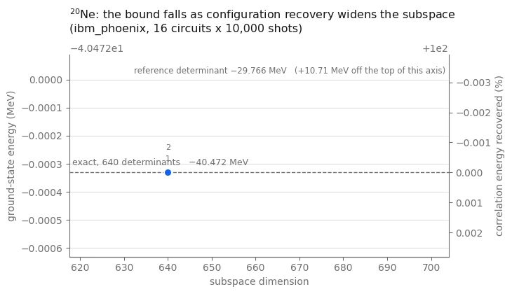
Malakihang halimbawa sa hardware

Ang pag-scale up ay nagbabago lamang ng mga input, kaya ang susunod na hakbang ay pagsamahin ang apat na stage sa isang function at patakbuhin ito nang dalawang beses, pareho sa isang 40-qubit na register sa $pf$ shell sa itaas ng $^{40}\mathrm{Ca}$ core gamit ang GXPF1 interaction [3].

Ang dalawang run ay nagpapakita ng iba't ibang aspekto ng scaling:

• Ang $^{44}\mathrm{Ti}$, dalawang valence proton at dalawang valence neutron, ay may 4,000-determinant basis. Ang register ay 40 qubits, pero maliit pa rin ang problema para ma-diagonalize nang eksakto sa isang laptop, kaya maikukumpara mo ang resulta ng hardware sa exact reference matapos palakihin ang laki ng register.

• Ang $^{48}\mathrm{Cr}$, apat na valence proton at apat na valence neutron, ay may 1,963,461 symmetry-allowed determinant sa parehong 40 qubits. Hindi ma-diagonalize ng dense solver ng tutorial ang buong space na iyon, kaya ang run ay nagbabalik ng rigorous upper bound at ang reference determinant na pinabuti nito.

Obserbahan ang dalawang dami sa dalawang run. Ang porsyento ng pool na kasya sa loob ng fixed gate budget ay lumiliit habang lumalaki ang pool, at inuulat ng pack_ensemble kung gaano karami ang kasama. Ang subspace ay hindi na nililimitahan ng sampling at nagsisimulang limitahan ng MAX_DIMENSION, ang pinakamalaking matrix na binubuo ng dense classical solver dito. Sa sukat na ito, gagamit ang isang production calculation ng selected configuration interaction (selected-CI) solver.

Pagsamahin ang hakbang 1–4

Tinatawag ng sumusunod na function ang parehong mga stage tulad ng walkthrough, sa parehong pagkakasunod-sunod.

def sqd_run(snt_file, n_protons, n_neutrons, name, exact=True):
    """The whole workflow for one nucleus.  Returns a record of every stage."""
    # -------------------------Step 1-------------------------
    ms = read_snt(DATA / snt_file, n_protons, n_neutrons)
    sp = m_scheme_states(ms)
    inter = Interaction(ms, sp)
    if sum(1 for s in sp if s.tz == -1) * 2 != len(sp):
        raise ValueError(
            f"{name}: post-selection needs equal proton and neutron state counts"
        )
    reference = reference_determinant(sp, inter, n_protons, n_neutrons)
    e_ref = matrix_element(inter, reference, reference)

    raw = excitation_pool(sp, reference)
    ranked = rank_pool(
        inter, reference, [op for op in raw if conserves_symmetry(sp, op)]
    )
    print(
        f"{name}: {len(sp)} qubits, {n_protons}p + {n_neutrons}n, A = {ms.mass_number}"
    )
    print(
        f"  2p2h pool {len(raw)} raw -> {len(ranked)} symmetry-allowed; "
        f"reference energy {e_ref:.6f} MeV"
    )

    # -------------------------Step 2-------------------------
    costs = excitation_costs(len(sp), ranked, costing_manager)
    circuits, bins, isa = pack_to_budget(
        len(sp),
        reference,
        ranked,
        costs,
        DEPTH_BUDGET,
        N_CIRCUITS,
        pass_manager,
    )
    packed = sum(len(b) for b in bins)
    worst = max(two_qubit_depth(c) for c in isa)
    worst_count = max(two_qubit_count(c) for c in isa)
    print(
        f"  packed {packed} of {len(ranked)} excitations; worst circuit two-qubit depth "
        f"{worst}, {worst_count} two-qubit gates"
    )

    # -------------------------Step 3-------------------------
    # a unique tag per run, so the jobs are findable later
    bit_arrays = sample(isa, SHOTS, JOB_TAGS + [name])
    matrix, probabilities, shots = pool_samples(bit_arrays, sp)
    survival = float(
        probabilities[
            (matrix[:, len(sp) // 2 :].sum(axis=1) == n_protons)
            & (matrix[:, : len(sp) // 2].sum(axis=1) == n_neutrons)
        ].sum()
    )
    print(
        f"  {shots:,} shots -> {len(matrix):,} distinct bitstrings, "
        f"{survival:.1%} of shots with the right nucleon numbers"
    )
    if survival == 0.0:
        raise RuntimeError(
            f"{name}: no shot carried the right nucleon numbers"
        )

    # -------------------------Step 4-------------------------
    result = recovery_loop(
        inter,
        sp,
        matrix,
        probabilities,
        reference,
        n_protons,
        n_neutrons,
        max_iterations=4,
        max_dimension=MAX_DIMENSION,
        seed=42,
    )
    energy = result["energy"]

    full_dim = count_basis(sp, n_protons, n_neutrons)  # cheap, even when huge
    e_exact = None
    if exact:
        full = full_basis(sp, n_protons, n_neutrons)
        if len(full) != full_dim:
            raise AssertionError(
                f"{name}: counted {full_dim} determinants but enumerated "
                f"{len(full)}"
            )
        e_exact, _ = ground_state(inter, full)

    print(f"  reference {e_ref:11.6f} MeV     pooled SQD {energy:11.6f} MeV")
    if e_exact is not None:
        print(
            f"  exact     {e_exact:11.6f} MeV  (dimension {full_dim})  ->  "
            f"{100 * (energy - e_ref) / (e_exact - e_ref):.1f}% of the correlation energy"
        )
        if energy < e_exact - 1e-7:
            raise AssertionError(
                f"{name}: pooled SQD bound is below the exact energy"
            )
    else:
        print(
            f"  no exact reference: the symmetry-allowed basis is {full_dim:,} determinants"
        )
        print(
            f"  the bound captures {energy - e_ref:.6f} MeV of correlation energy"
        )
    print()

    return dict(
        name=name,
        qubits=len(sp),
        pool=len(ranked),
        packed=packed,
        two_qubit=worst,
        two_qubit_gates=worst_count,
        shots=shots,
        distinct=len(matrix),
        survival=survival,
        dimension=len(result["basis"]),
        full_dim=full_dim,
        e_ref=e_ref,
        e_sqd=energy,
        e_exact=e_exact,
        history=result["history"],
        # the subspace and its eigenvector cannot be reconstructed from the summary --
        # they depend on the sampled shots -- so keep them for the scaling analysis
        interaction=inter,
        states=sp,
        reference=reference,
        ranked=ranked,
        basis=result["basis"],
        vector=result["vector"],
    )

pretty = {"20Ne": "$^{20}$Ne", "44Ti": "$^{44}$Ti", "48Cr": "$^{48}$Cr"}

small_scale = dict(
    name="20Ne",
    qubits=len(sp_sd),
    pool=len(ranked_sd),
    packed=PACKED_SD,
    two_qubit=worst_sd,
    two_qubit_gates=worst_count_sd,
    shots=shots_sd,
    distinct=len(matrix_sd),
    survival=shot_survival_sd,
    dimension=len(result_sd["basis"]),
    full_dim=len(basis_exact_sd),
    e_ref=E_REF_SD,
    e_sqd=E_SQD_SD,
    e_exact=E_EXACT_SD,
    history=result_sd["history"],
    interaction=inter_sd,
    states=sp_sd,
    reference=occ_sd,
    ranked=ranked_sd,
    basis=result_sd["basis"],
    vector=result_sd["vector"],
)

$^{44}\mathrm{Ti}$: ang parehong workflow sa isang 40-qubit na register

Ang $pf$ shell sa itaas ng $^{40}\mathrm{Ca}$ ay may apat na orbital bawat species at 20 magnetic substate bawat isa, kaya ang register ay 40 qubits. Dalawang valence proton at dalawang valence neutron ang bumubuo sa $^{44}\mathrm{Ti}$, na may 4,000 symmetry-allowed determinant — humigit-kumulang anim na beses ang $^{20}\mathrm{Ne}$ basis, gamit ang 40 qubits sa halip na 24.

Ito ang mas malaki sa dalawang halimbawa na maaaring lutasin nang eksakto ng notebook, kaya maikukumpara mo ang resulta ng hardware sa exact reference.

large_scale_verified = sqd_run("gxpf1.snt", 2, 2, "44Ti", exact=True)

44Ti: 40 qubits, 2p + 2n, A = 44
  2p2h pool 1602 raw -> 174 symmetry-allowed; reference energy -44.309387 MeV
  packed 96 of 174 excitations; worst circuit two-qubit depth 272, 285 two-qubit gates
job dap31a02fm4c73f67dp0: 16 circuits x 10,000 shots on ibm_phoenix
  160,000 shots -> 48,170 distinct bitstrings, 18.6% of shots with the right nucleon numbers
  iteration 1: 187 proton x 189 neutron halves -> dimension 3891, E = -47.849086 MeV
  iteration 2: 190 proton x 190 neutron halves -> dimension 4000, E = -47.876666 MeV
  iteration 3: 190 proton x 190 neutron halves -> dimension 4000, E = -47.876666 MeV
  reference  -44.309387 MeV     pooled SQD  -47.876666 MeV
  exact      -47.876666 MeV  (dimension 4000)  ->  100.0% of the correlation energy

$^{48}\mathrm{Cr}$: lampas sa kapasidad ng eksaktong diagonalization ng tutorial

Ang pagdaragdag ng dalawang proton at dalawang neutron ay gumagamit ng parehong 40-qubit na register (4, 4 para sa $^{48}\mathrm{Cr}$) at pinapataas ang laki ng basis nang halos 491 beses, sa 1,963,461 symmetry-allowed determinant. Ang matrix na iyon ay malayong-malayo sa kahit anong bubuuin ng tutorial na ito, kaya exact=False: walang eksaktong reference energy, kundi ang variational bound lamang at ang reference determinant na pinabuti nito.

May dalawang bagay na nagbabago sa sukat na ito, at parehong nakikita sa printout. Lumalaki ang pool sa ilang daang allowed excitation, kaya ang fixed gate budget ay sumasaklaw na lamang ng minorya nito sa halip na lahat nito. Gayundin, ang product subspace na sinasaklaw ng samples ay mas malaki kaysa sa MAX_DIMENSION, kaya tinatapyas ito ng dense solver ayon sa sampled weight. Nananatiling rigorous ang bound pero maaaring hindi kasingtumpak ng bound na kinalkula mula sa lahat ng sampled configuration. Ang production calculation ay pananatilihin ang samples at gagamit ng solver na sumusuporta sa mas malaking subspace.

large_scale_unverified = sqd_run("gxpf1.snt", 4, 4, "48Cr", exact=False)

48Cr: 40 qubits, 4p + 4n, A = 48
  2p2h pool 5536 raw -> 582 symmetry-allowed; reference energy -93.041237 MeV
  packed 96 of 582 excitations; worst circuit two-qubit depth 224, 279 two-qubit gates
job dap32a02fm4c73f67eog: 16 circuits x 10,000 shots on ibm_phoenix
  160,000 shots -> 55,436 distinct bitstrings, 18.6% of shots with the right nucleon numbers
  iteration 1: 223 proton x 223 neutron halves -> dimension 3977, E = -96.481598 MeV
  iteration 2: 223 proton x 223 neutron halves -> dimension 3977, E = -96.481598 MeV
  reference  -93.041237 MeV     pooled SQD  -96.481598 MeV
  no exact reference: the symmetry-allowed basis is 1,963,461 determinants
  the bound captures -3.440361 MeV of correlation energy

Suriin ang resulta na walang eksaktong reference

Ang run ng $^{48}\mathrm{Cr}$ ay walang eksaktong reference sa loob ng tutorial na ito. Gamitin ang mga umiiral na sample para suriin ang convergence at ikumpara sa classical selection baseline, nang walang dagdag na QPU time o full-space diagonalization.

Nakumberhe na ba ito? Kung i-reorder ang mga natirang determinant ayon sa kanilang weight sa nakumberhe nang eigenvector, magiging nested ang mga subspace, kaya ang pag-diagonalize sa nangungunang $d \times d$ block para sa isang hagdan na may $d$ ay sumusundan sa pagbaba ng bound sa dalawang dekada ng laki ng subspace. Kung matarik pa itong bumababa sa pinakamalaking $d$, ang dimension cap ng classical solver ang binding constraint at MAX_DIMENSION ang parameter na dapat dagdagan. Kung patag na ito, kaunti lang ang maidudulot ng dagdag na natirang determinant; maaaring kailanganin ang pag-sample ng karagdagang configuration para sa karagdagang progreso. Ang Hamiltonian ay binubuo isang beses sa buong laki at bawat rung ay isang principal block nito, kaya ang buong sweep ay nagkakahalaga ng isang matrix build sa halip na isa bawat rung.

Paano ihahambing ang quantum sampling sa classical selection? Ikumpara sa isang subspace ng parehong laki na napili ng classical selection procedure: kunin ang pool na naka-rank ayon sa perturbation theory sa score order, palakihin ang product subspace sa parehong dimension, at i-diagonalize iyon sa halip. Parehong curve ay rigorous upper bound sa parehong Hamiltonian, kaya kung alin man ang mas mababa sa parehong dimension ang pumili ng mas magandang determinant. Ang paghahambing na ito ang magpapasya kung pinapabuti ng hardware sampling ang energy estimate kumpara sa classical baseline na ito.

Hindi napili ang subspace na ito para sa excited states. Ginagabayan ng configuration recovery ang subspace gamit ang ground-state occupancies, kaya ang mga mas mataas na eigenvalue ay mas malayo pa sa convergence kaysa sa pinakamababa, at ang unang excitation energy ay lumalabas na mas mataas kaysa sa sinusukat na $2^+$. Para maabot nang maayos ang excited states, kailangan ng subspace na piniling talaga para dito.

def subspace_scaling(
    inter, basis, vector, points=18, smallest=32, largest=None
):
    """Nested Rayleigh-Ritz sweep: the lowest eigenvalue of the leading d x d block, for a ladder of d.

    Reordering the basis by descending weight in the converged eigenvector makes every subspace in
    the ladder a subset of the next, so the energies fall monotonically and each one is a valid
    variational bound.  H is built once at full size; each rung is a principal block.
    """
    order = np.argsort(-(np.abs(vector) ** 2))
    ordered = [basis[i] for i in order]
    weights = (np.abs(vector) ** 2)[order]
    if (
        largest is not None
    ):  # cap the ladder so two subspaces end at a common dimension
        ordered, weights = ordered[:largest], weights[:largest]
    H = subspace_hamiltonian(inter, ordered)
    dimensions = np.unique(
        np.geomspace(smallest, len(ordered), points).astype(int)
    )
    rows = [
        (
            int(d),
            float(
                eigh(H[:d, :d], eigvals_only=True, subset_by_index=[0, 0])[0]
            ),
        )
        for d in dimensions
    ]
    return rows, np.cumsum(weights)

def classical_selection(
    inter, sp, reference, ranked, target, n_protons, n_neutrons
):
    """The subspace classical perturbative ranking would pick, grown to `target` dimension.

    Same product construction as the sampled subspace, and the same truncation discipline -- half
    configurations are offered to `grow_subspace` in order of importance and it takes as many as
    fit.  The only difference from the sampled path is where the ordering comes from: PT2 score
    here, measured sampling weight there.  So the comparison isolates *which determinants got
    chosen* and nothing else.

    Truncating by any other rule would not be a fair baseline.  Slicing an arbitrarily ordered
    list, for instance, keeps determinants by accident rather than by importance and makes the
    classical subspace look worse than classical selection really is.
    """
    p_ref = tuple(i for i in reference if sp[i].tz == -1)
    n_ref = tuple(i for i in reference if sp[i].tz == +1)
    reached = {reference}
    proton_order, neutron_order = [p_ref], [n_ref]
    seen_p, seen_n = {p_ref}, {n_ref}
    product_budget = 4 * target

    for op, _, _ in ranked:  # ranked is already in descending PT2 score
        h1, h2, v1, v2 = op
        fresh = {
            tuple(sorted(set(d) - {h1, h2} | {v1, v2}))
            for d in reached
            if {h1, h2} <= set(d) and not {v1, v2} & set(d)
        }
        reached |= fresh
        for det in fresh:  # first appearance fixes a half's rank
            half_p = tuple(i for i in det if sp[i].tz == -1)
            half_n = tuple(i for i in det if sp[i].tz == +1)
            if half_p not in seen_p:
                seen_p.add(half_p)
                proton_order.append(half_p)
            if half_n not in seen_n:
                seen_n.add(half_n)
                neutron_order.append(half_n)
        if len(proton_order) * len(neutron_order) > product_budget:
            # Half-configuration products over-count the subspace, because only the
            # symmetry-allowed ones survive `product_subspace`.  Stopping on the product
            # count alone can therefore leave the basis far short of `target`, so check
            # the dimension actually realized and widen the budget if it falls short.
            trial, _, _ = grow_subspace(
                sp,
                [p_ref],
                [n_ref],
                proton_order,
                neutron_order,
                n_protons,
                n_neutrons,
                max_dimension=target,
            )
            if len(trial) >= target:
                break
            product_budget *= 2

    basis, _, _ = grow_subspace(
        sp,
        [p_ref],
        [n_ref],
        proton_order,
        neutron_order,
        n_protons,
        n_neutrons,
        max_dimension=target,
    )
    return basis

run = large_scale_unverified
if "basis" not in run:
    raise RuntimeError(
        "this cell needs the subspace and eigenvector that sqd_run now returns; "
        "re-run the sqd_run definition and the 48Cr cell"
    )

print(
    f"{run['name']}: sweeping nested subspaces of the sampled basis "
    f"(dimension {run['dimension']})"
)
sampled_rows, cumulative = subspace_scaling(
    run["interaction"], run["basis"], run["vector"]
)

print(
    f"{run['name']}: building the classically selected subspace at the same dimension"
)
classical_basis = classical_selection(
    run["interaction"],
    run["states"],
    run["reference"],
    run["ranked"],
    run["dimension"],
    4,
    4,
)
# Both subspaces must be scored at the same dimension.  Symmetry filtering can still leave
# the classical construction short of the target when the ranked pool runs out, so take the
# dimension both actually reach, cap both ladders there, and verify they agree.
common_dim = min(sampled_rows[-1][0], len(classical_basis))
if common_dim < sampled_rows[-1][0]:
    sampled_rows, _ = subspace_scaling(
        run["interaction"], run["basis"], run["vector"], largest=common_dim
    )
classical_rows, _ = subspace_scaling(
    run["interaction"],
    classical_basis,
    ground_state(run["interaction"], classical_basis)[1],
    largest=common_dim,
)
if sampled_rows[-1][0] != classical_rows[-1][0]:
    raise RuntimeError(
        f"comparison dimensions differ: sampled {sampled_rows[-1][0]}, "
        f"classical {classical_rows[-1][0]}"
    )

advantage = sampled_rows[-1][1] - classical_rows[-1][1]
direction = "lower" if advantage < 0 else "higher"
verdict = "beats" if advantage < 0 else "does not beat"
descent = next(
    e for d, e in reversed(sampled_rows) if d <= sampled_rows[-1][0] / 2
)
for fraction in (0.90, 0.99):
    count = int(np.searchsorted(cumulative, fraction) + 1)
    print(
        f"  {fraction:.0%} of the eigenvector norm sits on {count} determinants "
        f"({count / run['full_dim']:.1e} of the {run['full_dim']:,}-determinant space)"
    )
print(
    f"  bound still falling {1000 * (sampled_rows[-1][1] - descent):+.1f} keV "
    f"over the last doubling of dimension"
)
print(
    f"  sampled {sampled_rows[-1][1]:.6f} MeV vs classically selected "
    f"{classical_rows[-1][1]:.6f} MeV at a verified common dimension of "
    f"{classical_rows[-1][0]:,}"
)
print(
    f"  -> the sampled subspace is {abs(advantage) * 1000:.0f} keV {direction}"
)

48Cr: sweeping nested subspaces of the sampled basis (dimension 3977)
48Cr: building the classically selected subspace at the same dimension
  90% of the eigenvector norm sits on 107 determinants (5.4e-05 of the 1,963,461-determinant space)
  99% of the eigenvector norm sits on 593 determinants (3.0e-04 of the 1,963,461-determinant space)
  bound still falling -15.6 keV over the last doubling of dimension
  sampled -96.481598 MeV vs classically selected -95.314510 MeV at a verified common dimension of 3,957
  -> the sampled subspace is 1167 keV lower

fig, axes = plt.subplots(1, 2, figsize=(11.2, 4.0), facecolor=SURFACE)

# left: two nested convergence curves on the same axes
ax = axes[0]
ax.set_facecolor(SURFACE)
ax.plot(
    [d for d, _ in sampled_rows],
    [e for _, e in sampled_rows],
    "-o",
    color=SERIES,
    linewidth=2,
    markersize=5,
    markeredgecolor=SURFACE,
    markeredgewidth=1,
    zorder=4,
    label="sampled on the QPU",
)
ax.plot(
    [d for d, _ in classical_rows],
    [e for _, e in classical_rows],
    "--s",
    color=MUTED,
    linewidth=1.6,
    markersize=4,
    markeredgecolor=SURFACE,
    markeredgewidth=1,
    zorder=3,
    label="classically selected, same size",
)
ax.axhline(run["e_ref"], color=RULE, linestyle=":", linewidth=1.2, zorder=1)
ax.annotate(
    f"reference determinant {run['e_ref']:.2f} MeV".replace("-", "\u2212"),
    xy=(sampled_rows[-1][0], run["e_ref"]),
    xytext=(-2, 4),
    textcoords="offset points",
    ha="right",
    va="bottom",
    color=MUTED,
    fontsize=8,
)

# mark the gap between the two curves at the largest dimension, not either curve alone
edge = sampled_rows[-1][0]
ax.plot(
    [edge, edge],
    [classical_rows[-1][1], sampled_rows[-1][1]],
    "-",
    color=SERIES,
    linewidth=1.0,
    alpha=0.7,
    zorder=2,
)
ax.annotate(
    f"{abs(advantage) * 1000:.0f} keV {direction}\nat equal dimension",
    xy=(edge, 0.5 * (classical_rows[-1][1] + sampled_rows[-1][1])),
    xytext=(-8, 0),
    textcoords="offset points",
    ha="right",
    va="center",
    color=SERIES,
    fontsize=8.5,
)

ax.set_xscale("log")
ax.set_xlim(sampled_rows[0][0] * 0.75, edge * 1.5)
ax.set_xlabel("subspace dimension", color=MUTED)
ax.set_ylabel("variational upper bound (MeV)", color=MUTED)
ax.set_title(
    f"{pretty[run['name']]}: the bound, and the subspace it {verdict}",
    color=INK,
    fontsize=11,
    loc="left",
    pad=10,
)
legend = ax.legend(frameon=False, fontsize=8.5, loc="lower left")
for text in legend.get_texts():
    text.set_color(MUTED)

# right: why a few thousand determinants can bound two million
ax = axes[1]
ax.set_facecolor(SURFACE)
ranks = np.arange(1, len(cumulative) + 1)
ax.plot(ranks, 100 * cumulative, "-", color=DEEP, linewidth=2, zorder=3)
for fraction, style, label_y in ((0.90, ":", 46), (0.99, "--", 24)):
    count = int(np.searchsorted(cumulative, fraction) + 1)
    ax.axvline(count, color=MUTED, linestyle=style, linewidth=1, zorder=1)
    ax.annotate(
        f"{fraction:.0%} of the norm\non {count} determinants",
        xy=(count, label_y),
        xytext=(7, 0),
        textcoords="offset points",
        ha="left",
        va="center",
        color=MUTED,
        fontsize=8.5,
    )
ax.set_xscale("log")
ax.set_xlim(0.8, len(cumulative) * 2.6)
ax.set_ylim(0, 104)
ax.set_xlabel("determinants, ordered by weight", color=MUTED)
ax.set_ylabel("cumulative share of the eigenvector (%)", color=MUTED)
ax.set_title(
    f"Sparsity: {run['full_dim']:,} determinants in the sector",
    color=INK,
    fontsize=11,
    loc="left",
    pad=10,
)

for ax in axes:
    ax.grid(axis="y", color=RULE, alpha=0.55)
    ax.tick_params(colors=MUTED, labelsize=8.5)
    for side in ("top", "right"):
        ax.spines[side].set_visible(False)
    for side in ("bottom", "left"):
        ax.spines[side].set_color(MUTED)
fig.tight_layout()
plt.show()

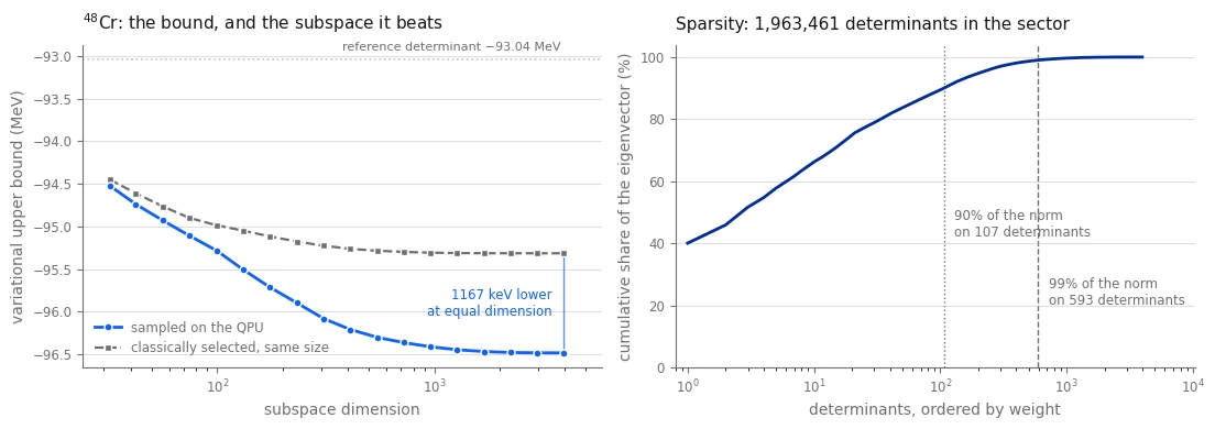
Ikumpara ang tatlong run

Hindi maikukumpara ang absolute energies sa iba't ibang nuclei at interactions, kaya tumutok sa porsyento ng correlation energy na nabawi sa mga run, kung saan may eksaktong reference. Ikumpara din ang circuit depth at ang porsyento ng mga shot na itinapon.

runs = [small_scale, large_scale_verified, large_scale_unverified]

print(
    f"{'run':>6}  {'qubits':>6}  {'pool':>9}  {'2q depth':>8}  {'2q gates':>8}  "
    f"{'shots kept':>10}  {'dim':>6}  {'of':>9}  {'% corr':>7}"
)
for r in runs:
    fraction = (
        "--"
        if r["e_exact"] is None
        else f"{100 * (r['e_sqd'] - r['e_ref']) / (r['e_exact'] - r['e_ref']):.1f}%"
    )
    coverage = "{}/{}".format(r["packed"], r["pool"])
    print(
        f"{r['name']:>6}  {r['qubits']:>6}  {coverage:>9}  "
        f"{r['two_qubit']:>8}  {r['two_qubit_gates']:>8}  {r['survival']:>9.1%}  "
        f"{r['dimension']:>6}  {(r['full_dim'] or 0):>9,}  {fraction:>7}"
    )

print()
for r in runs:
    exact = (
        f"exact {r['e_exact']:11.6f}"
        if r["e_exact"] is not None
        else "exact  unavailable"
    )
    print(
        f"{r['name']:>6}   reference {r['e_ref']:11.6f}   pooled SQD {r['e_sqd']:11.6f}   {exact} MeV"
    )

run  qubits       pool  2q depth  2q gates  shots kept     dim         of   % corr
  20Ne      24      78/78       228       234      31.5%     640        640   100.0%
  44Ti      40     96/174       272       285      18.6%    4000      4,000   100.0%
  48Cr      40     96/582       224       279      18.6%    3977  1,963,461       --

  20Ne   reference  -29.765549   pooled SQD  -40.472331   exact  -40.472331 MeV
  44Ti   reference  -44.309387   pooled SQD  -47.876666   exact  -47.876666 MeV
  48Cr   reference  -93.041237   pooled SQD  -96.481598   exact  unavailable MeV

# Left: how much of the correlation energy was recovered, where the exact answer is known.
# Right: the bound itself for the run that has nothing to score against.
scored = [r for r in runs if r["e_exact"] is not None]

fig, ax = plt.subplots(figsize=(6.4, 3.9), facecolor=SURFACE)
ax.set_facecolor(SURFACE)
labels = [
    f"{pretty[r['name']]}\n{r['qubits']} qubits\n{r['full_dim']:,} determinants"
    for r in scored
]
fractions = [
    100 * (r["e_sqd"] - r["e_ref"]) / (r["e_exact"] - r["e_ref"])
    for r in scored
]
shades = [SERIES, DEEP, PURPLE]
bars = ax.bar(
    labels, fractions, width=0.46, color=shades[: len(scored)], zorder=3
)
for bar, fraction, r in zip(bars, fractions, scored):
    ax.annotate(
        f"{fraction:.1f}%",
        xy=(bar.get_x() + bar.get_width() / 2, fraction),
        xytext=(0, 5),
        textcoords="offset points",
        ha="center",
        va="bottom",
        color=INK,
        fontsize=10,
    )
    ax.annotate(
        f"dim {r['dimension']:,}",
        xy=(bar.get_x() + bar.get_width() / 2, 3),
        ha="center",
        va="bottom",
        color=SURFACE,
        fontsize=8.5,
    )
ax.axhline(100, color=MUTED, linestyle="--", linewidth=1, zorder=1)
ax.annotate(
    "exact diagonalization",
    xy=(-0.45, 100),
    xytext=(0, 4),
    textcoords="offset points",
    ha="left",
    va="bottom",
    color=MUTED,
    fontsize=8.5,
)
ax.set_ylim(0, 118)
ax.set_ylabel("correlation energy recovered (%)", color=MUTED)
ax.set_title(
    f"Where the exact answer is known ({backend.name})",
    color=INK,
    fontsize=11,
    loc="left",
    pad=10,
)
ax.grid(axis="y", color=RULE, alpha=0.55)
ax.tick_params(colors=MUTED, labelsize=8.5)
for side in ("top", "right"):
    ax.spines[side].set_visible(False)
for side in ("bottom", "left"):
    ax.spines[side].set_color(MUTED)
fig.tight_layout()
plt.show()

# the same convergence view as the walkthrough, for the run with no exact reference
convergence_plot(
    large_scale_unverified["history"],
    large_scale_unverified["e_ref"],
    None,
    f"{pretty[large_scale_unverified['name']]}: "
    f"{large_scale_unverified['full_dim']:,} determinants, no exact answer to score against\n"
    f"({backend.name}, {N_CIRCUITS} circuits x {SHOTS:,} shots)",
    colour=DEEP,
)
plt.show()

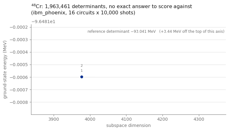
Buod

Isang workflow, walang pagbabago maliban sa mga input nito, ang tumakbo sa isang QPU sa tatlong laki ng problema: isang 24-qubit na problema na masusuri mo nang eksakto, isang 40-qubit na problema na masusuri mo pa rin nang eksakto, at isang 40-qubit na problema na may halos dalawang milyong basis states na lampas sa kapasidad ng eksaktong diagonalization ng tutorial na ito.

Ang tatlong run ay nagpapakita ng mga sumusunod na punto:

• Ang tanging kailangang gawin ng quantum step ay magmungkahi ng mga determinant. Fixed ang circuit, na sinimulan mula sa second-order perturbation theory, at hindi kailanman na-optimize. Wala sa workflow ang nangangailangan na tumpak ang mga amplitude nito, tanging kailangan lang ay maging kapaki-pakinabang ang support nito. Ang classical diagonalization sa napiling subspace ay nagbibigay ng variational upper bound, bagama't nag-iiba ang bound ayon sa mga sampled configuration.

• Binabawasan ng qubit excitations ang circuit depth. Dahil ang support lang ang mahalaga, ang fermionic excitation blocks ay maaaring palitan ng qubit excitations, na ang gastos ay hindi lumalaki kasabay ng distansya sa pagitan ng mga orbital na kinokonekta nito. Sinukat ng Hakbang 2 ang pagtitipid sa aktwal na backend, na siyang pagkakaiba sa pagitan ng isang circuit na maayos na kasya sa loob ng coherence at isang hindi.

• Ginagamit muli ng configuration recovery ang maingay na samples. Bawat shot na may maling bilang ng proton o neutron ay inaayos laban sa kasalukuyang estimate ng occupancy sa halip na itapon, at bawat inayos na half-configuration ay maaaring magdagdag ng configuration sa subspace. Ang pagpapalawak ng variational subspace ay hindi maaaring magpataas ng pinakamababang eigenvalue nito. Ipinapakita ng tutorial na ito ang configuration recovery gamit ang hardware samples.

• Lumilipat ang binding constraint habang nag-scale ka. Sa 24 qubits, kaya ng ansatz na maabot ang eksaktong sagot, at ang sampling lamang ang naging hadlang. Sa 40 qubits na may apat na valence nucleon bawat species, ang gate budget ay sumasaklaw lamang ng minorya ng pool at nililimitahan ng dense classical solver ang subspace. Ang pag-alam kung alin sa tatlo ang naglilimita sa iyo ang praktikal na kasanayan na itinuturo ng workflow na ito.

Mga susunod na hakbang

Mga Rekomendasyon

Galugarin ang mga kaugnay na resource na ito:

• Sample-based quantum diagonalization ng isang chemistry Hamiltonian: ang parehong algorithm na inilapat sa electronic structure, gamit ang selected-CI solver ng SQD addon.

• Dokumentasyon ng SQD addon: post-selection, subsampling, at configuration-recovery utilities.

• Mga algorithm sa quantum diagonalization: isang buong course sa subspace diagonalization, kasama ang Krylov variants.

• Panimula sa transpilation: ang mga opsyon ng pass-manager na mahalaga kapag ang isang circuit ay dominado ng two-qubit gates.

• Mga execution mode: galugarin ang batch mode para sa pag-iskedyul ng mga independent na job.

Mga extension na dapat isaalang-alang

• Palitan ang dense solver. Ang MAX_DIMENSION ang siyang hangganan ng lahat sa sukat ng $^{48}\mathrm{Cr}$, at ang np.linalg.eigh sa isang dense matrix ang dahilan nito. Ang pagbuo ng parehong projected Hamiltonian bilang isang sparse matrix at paggamit ng iterative eigensolver tulad ng scipy.sparse.linalg.eigsh, o isang Davidson o selected-CI solver na dinisenyo para sa nuclear two-body interaction, ay maaaring sumuporta sa mas malaking subspace. Nakadepende ang praktikal na hangganan sa sparsity ng matrix, available na memory, at convergence ng solver, at hindi sinusuri ng tutorial na ito ang extension na iyon. Ang qiskit_addon_sqd.fermion.solve_sci ng SQD addon ay hindi drop-in substitute: binabalot nito ang isang electronic-structure solver at umaasa ng one- at two-body integrals sa anyong iyon, kaya ang shared proton $\times$ neutron product structure ay hindi sapat nang mag-isa. Ang paggamit nito ay mangangahulugan ng pag-map sa shell-model interaction ng Equation (1) papunta sa mga integrals na iyon at ang pagvalidate ng resulta laban sa eksaktong energies na kinakalkula na ng notebook na ito.

• Magdagdag ng batching at subsampling. Ang published pooled SQD workflow ay nagda-diagonalize ng ilang independent subsample bawat iteration at kinukuha ang pinakamahusay. Ang tutorial na ito ay gumagamit ng isang batch bawat iteration, na walang epekto sa variational bound pero hindi nagbibigay ng variance information na nagpapahiwatig kung tutulong pa ang dagdag na shots.

• Excited states at iba pang sector. Ang mas mataas na eigenvalue ng bawat subspace Hamiltonian ay upper bound sa excited states sa parehong symmetry sector, at ang pagpapatakbo sa $M_J \neq 0$ ay umaabot sa ibang sector. Ang $2^+$ check sa Hakbang 1 ay kalahati na ng kalkulasyong ito.

• Isang cross-shell model space. Awtomatikong nasusunod ang parity sa loob ng isang major shell, kaya't wala itong ginagawang trabaho dito. Ang isang $sd$-$pf$ space ay naghahalo ng $\ell$ parities, na ginagawang tunay na ikaapat na constraint ang parity, isang bagay na hindi mahuhuli ng Hamming-weight repair ng SQD o ng product construction nang mag-isa.

• Mga odd-mass nucleus. Kinakailangan ng reference_determinant ang even valence count sa bawat species, dahil ang time-reversed paired filling ang nagpapataw ng $M_J = 0$. Kailangan ng odd nucleus ng half-integer $M_J$ target at unpaired reference.

Apendise

Ipinapaliwanag ng seksyong ito ang katuwiran sa likod ng mga helper na ipinakilala sa seksyong Setup.

Bakit hindi opsyonal ang mass-dependence rescaling

Ang empirical shell-model interactions ay in-fit sa isang mass at inilapat sa buong chain ng isotopes, kasama ang two-body matrix elements na naka-scale bilang $(A/A_{\mathrm{ref}})^{p}$. Parehong interaction files ay may $p = -0.3$, na may $A_{\mathrm{ref}} = 18$ para sa USD family at $42$ para sa GXPF1. Sa two-body header line ng isang .snt file, ang dalawang numerong iyon ay nasa posisyon kung saan sana napupunta ang oscillator frequency at core energy, na ginagawa itong madaling malito; ang pagbasa sa exponent bilang isang constant core energy ay nagdaragdag ng katha-thang offset sa bawat diagonal element at nawawala ang rescaling, na nagpapabago sa correlation energy nang ilang porsyento. Ang symmetry check sa Hakbang 1 ay hindi sa kanyang sarili nagbebe-verify ng energy scale. Ang paghahambing sa $2^+$ excitation energy, na sinusukat sa MeV, kasama ang eksperimento ay nagbibigay ng karagdagang check sa mass-dependent rescaling. Ang excitation energy ay pagkakaiba sa pagitan ng mga level, kaya hindi nito nadedetect ang isang constant offset na inilapat sa lahat ng energies.

Bakit natagpuan sa pamamagitan ng search ang reference sa halip na sa pagpuno

Ang maliwanag na reference ay ang determinant na pumupuno sa pinakamababang single-particle energies. Hindi ito ang determinant na may pinakamababang energy, dahil ang diagonal ng Equation (1) ay may kasamang two-body term $\sum_{i<j} \langle ij \| ij \rangle$, at ang pairing interaction ay malakas na nagpapaboran ng pag-occupy sa time-reversed $(+m_j, -m_j)$ partners sa pinakamalaking available na $|m_j|$. Sa $sd$ shell, iyan ang pagkakaiba sa pagitan ng $m_j = \pm 1/2$ pair at $m_j = \pm 5/2$ pair ng $0d_{5/2}$, at nagkakahalaga ito ng mga 1 MeV; sa $pf$ shell, mas malapit ito sa 2. Dahil tinutukoy ng reference energy ang zero ng metric na "na-recover na correlation energy", ang mahinang pagpili ay nagpapalaki sa metric na iyon at nagbibigay ng mas hindi tumpak na simulang punto.

Ang paglimita sa paired fillings ay ginagawang mura ang exhaustive search, na may $\binom{n_{\mathrm{pairs}}}{k}$ candidates bawat species (ilang libo lamang ang maximum), at sinisiguro ang $M_J = 0$. Sa bawat kaso sa tutorial na ito na masusuri laban sa isang full enumeration, ibinabalik ng search ang global lowest-diagonal determinant, na siya ring pinakamalaking component ng eksaktong ground state.

Bakit ang first-order amplitude, hindi ang eksaktong two-level angle

Ang pag-diagonalize sa $2 \times 2$ Hamiltonian sa space $\{|\Phi_{\mathrm{ref}}\rangle, |\alpha\rangle\}$ ay nagbibigay ng mixing angle $\theta_{\mathrm{exact}} = \tfrac{1}{2}\arctan(2V/\Delta)$; maaaring matukso kang tawagin itong tamang pagpili para sa isang isolated na pares ng levels. Sa ansatz na ito, ilang dosenang excitation block ang kumikilos nang sunud-sunod sa parehong reference, kaya ang pag-optimize sa bawat block nang hiwalay ay hindi kinakailangang nag-optimize sa composite circuit.

Ang tungkulin ng circuit ang nagtatakda ng pagpili ng angle. Dahil $|\tfrac{1}{2}\arctan(2x)| \le |x|$ para sa bawat totoong $x$, ang eksaktong angle ay palaging mas maliit sa magnitude kaysa sa first-order amplitude na $t = V/\Delta$, at samakatuwid ay palaging nag-iiwan ng mas maraming amplitude sa reference determinant. Ang isang circuit na nagpapanatili ng mas maraming amplitude sa reference ay mas madalas na ibinabalik ang reference at mas bihira ang natatanging excited determinants. Para sa pooled SQD, ang kapaki-pakinabang na output ng isang shot ay isang determinant na hindi pa nakikita ng classical step, na siyang dahilan kung bakit ginagamit ang mas malaking angle sa tutorial na ito. Hindi kailangang maging tumpak ang alinman sa dalawang angle, dahil itinatapon nang buo ng classical diagonalization ang amplitude ng circuit at kinukuha ang sarili nitong bago.

Bakit magagamit ng pooled SQD ang qubit excitations

Ang fermionic excitation na $T = a_{v_1}^\dagger a_{v_2}^\dagger a_{h_2} a_{h_1}$ ay naka-map sa ilalim ng Jordan-Wigner sa walong Pauli strings, bawat isa'y may dalang $Z$ operators sa bawat qubit sa pagitan ng pinakalabas na indices. Ini-encode ng mga string na iyon ang fermionic sign, at lumalaki ang gastos nito kasabay ng span, na para sa isang proton-neutron excitation ay ang buong register.

Ang pagtanggal sa mga ito ay nagbibigay ng qubit-excitation operator ni Yordanov et al. [5]. Iba itong operator: naiiba ang state na inihahanda nito sa fermionic isa sa signs ng mga amplitude nito, at maaaring magkaiba nang malaki ang dalawang sampling distribution. Ang hindi nagbabago ay kung aling mga determinant ang may nonzero amplitude, dahil ang bawat block ay umiikot pa rin sa loob ng parehong two-dimensional space na $\{|d\rangle, |d'\rangle\}$ para sa bawat determinant na $d$ na kinikilusan nito, at pinapanatili pa rin nito ang parehong dalawang nucleon numbers, $M_J$, at parity nang eksakto. Kaya magkatulad ang reachable set ng determinants, at ang reachable set lamang ang ginagamit ng pooled SQD; ang classical diagonalization ay nagtatakda ng sarili nitong amplitudes kahit anuman. Sinusuri ng Hakbang 2 ang claim na magkatulad ang support sa isang totoong operator mula sa pool at sinusukat kung magkano ang natitipid ng substitution.

Ang limitasyon ay naiiba ang mga weight ng sampling, kaya hindi matutuklasan ng dalawang konstruksyon ang mga determinant sa parehong pagkakasunod-sunod sa finite shot count. Dahil ang ranking na nagpapasya kung aling excitations ang pumapasok sa mga circuit ay classical at hindi nagbabago, at ang classical step ay nagre-re-weight naman ng lahat, ang pagkakaiba sa sampling weights ay isang tradeoff para sa mas mababang circuit depth.

Bakit kabilang ang $M_J$ sa product stage

Ang post-selection at configuration recovery ay parehong kumikilos sa Hamming weights: ang bilang ng proton sa isang kalahati ng register, at ang bilang ng neutron sa kabila. Hindi kabilang sa anyong iyon ang $M_J = M_p + M_n$. Ito ay isang property ng isang proton configuration na naka-pares sa isang neutron configuration. Ang isang shot kung saan ang kalahati nitong proton at kalahati nitong neutron ay parehong may tamang bilang ng nucleon ay naglalaman ng dalawang magagamit na half-configuration kahit hindi nagkakansela ang kanilang mga $M_J$ value, dahil ganap na maganda ang proton half sa $M_p = +1$ kapag ipinares ito sa neutron half sa $M_n = -1$. Ang pag-filter ng buong shot batay sa total $M_J$ ay itinatapon ang dalawang kalahati, at ang pagpapataw ng $M_J$ sa mga pinagsamang produkto ay pinapanatili ang mga ito. Ang parehong argumento ang nagpapaliwanag kung bakit hindi kailangan ng recover_configurations ng konsepto ng $M_J$ para maging kapaki-pakinabang sa kasong ito.

Mga Reperensya

1. J. Robledo-Moreno, M. Motta, H. Haas, et al., "Chemistry beyond the scale of exact diagonalization on a quantum-centric supercomputer", Science Advances 11, eadu9991 (2025). arXiv:2405.05068

2. B. A. Brown and W. A. Richter, "New USD Hamiltonians for the sd shell", Physical Review C 74, 034315 (2006). Ang embedded na usda.snt file ay may dalang USDA parameters gaya ng na-tabulate ni W. A. Richter, S. Mkhize and B. A. Brown, "sd-shell observables for the USDA and USDB Hamiltonians", Physical Review C 78, 064302 (2008).

3. M. Honma, T. Otsuka, B. A. Brown and T. Mizusaki, "Effective interaction for pf-shell nuclei", Physical Review C 65, 061301(R) (2002).

4. B. Huron, J. P. Malrieu and P. Rancurel, "Iterative perturbation calculations of ground and excited state energies from multiconfigurational zeroth-order wavefunctions", The Journal of Chemical Physics 58, 5745 (1973).

5. Y. S. Yordanov, D. R. M. Arvidsson-Shukur and C. H. W. Barnes, "Efficient quantum circuits for quantum computational chemistry", Physical Review A 102, 062612 (2020).

6. National Nuclear Data Center, Evaluated Nuclear Structure Data File, Brookhaven National Laboratory. Pinagmulan ng sinusukat na $2^+$ excitation energies na binanggit sa Hakbang 1.