I-simulate ang neutron scattering gamit ang AQC + Trotter dynamics Serverless workflow
Tinatayang oras ng paggamit: 18 minuto sa isang Heron r3 processor (TANDAAN: Isa lang itong tantiya. Maaaring magkaiba ang aktwal na runtime.)
Mga natutunan
-
Paano nagma-map ang inelastic neutron-scattering spectrum sa dynamical structure factor ng 1D quantum magnet.
-
Paano ihahanda ang KCuF (isotropic Heisenberg) ground state gamit ang density matrix renormalization group (DMRG) at matrix product state (MPS) fidelity maximization.
-
Paano magpatakbo ng Trotter time-evolution, approximate quantum compilation (AQC) circuit compression, at mitigated execution bilang isang function call lamang.
-
Paano i-post-process ang per-site time series sa at tukuyin ang two-spinon continuum.
Mga paunang kailangan
-
Pagiging pamilyar sa Qiskit patterns,
SparsePauliOp, at Trotter time-evolution. -
Kapaki-pakinabang ngunit hindi kailangan ang pangunahing kaalaman sa tensor-network methods (DMRG at MPS), gayundin ang pagiging pamilyar sa
qiskit-addon-aqc-tensorna library na ginagamit ng function para i-compress ang mga Trotter circuit.
Background
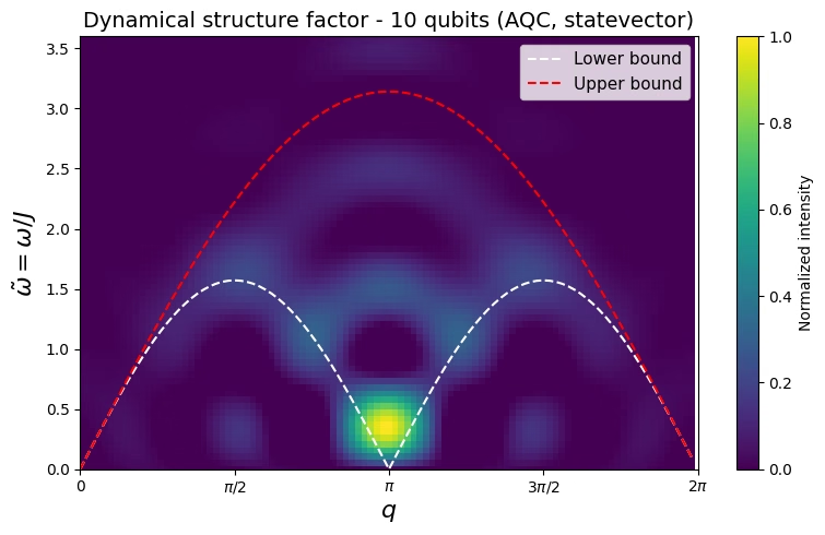
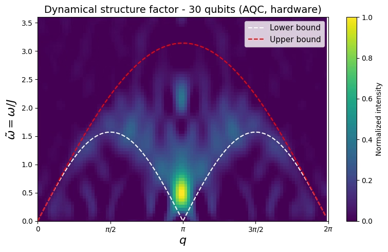
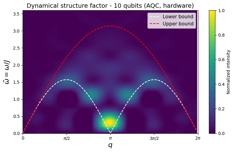
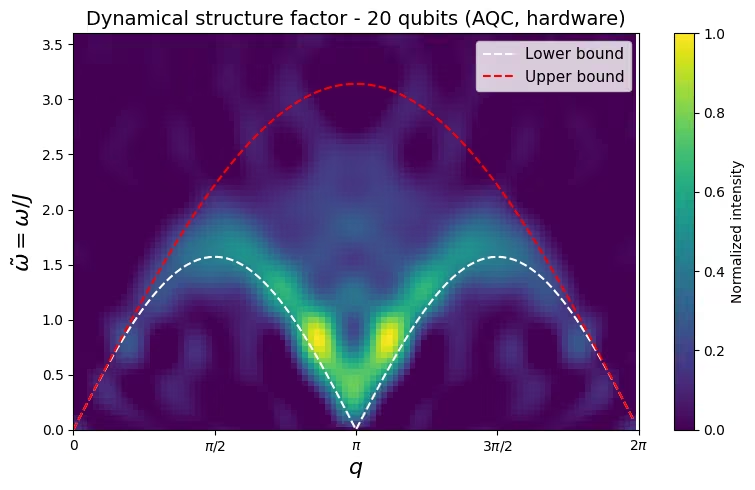
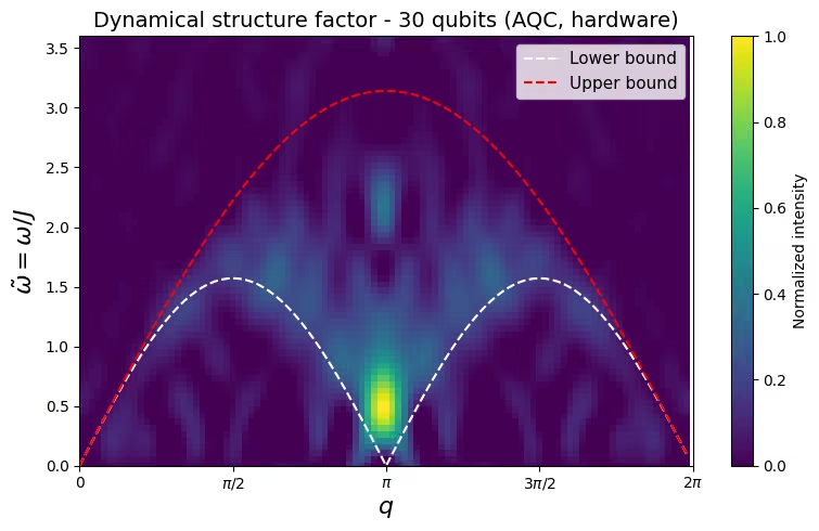
Sinusukat ng inelastic neutron scattering ang dynamical structure factor , ang space-and-time Fourier transform ng spin-spin correlation function, kaya ang pag-reproduce ng mula sa isang microscopic spin model ay isang direkta at falsifiable na pagsubok ng isang quantum simulation. Sinusuri ng tutorial na ito ang KCuF, isang spin- antiferromagnetic Heisenberg chain na ang mga excitation ay hindi single spin flips kundi mga pares ng fractionalized spinons: sa halip na matalim na magnon dispersion, ang ay nagpapakita ng malawak na two-spinon continuum, na hinahangganan sa ibaba ng at sa itaas ng . Iyon ang mga dashed curve sa mga plot na susunod. Ang pisika sa kabuuan, at ang paghahambing laban sa sinukat na neutron data, ay sinasaklaw sa orihinal na tutorial at sa Lee et al., arXiv:2603.15608.
Sinasalamin ng quantum workflow ang scattering experiment:
-
Ihanda ang ground state ng chain .
-
Sipahin ito ng local perturbation sa gitnang site, isang -rotation, na ginagaya ang paglipat ng momentum at enerhiya mula sa neutron.
-
I-time-evolve sa ilalim ng Heisenberg Hamiltonian, , gamit ang Trotter product formula.
-
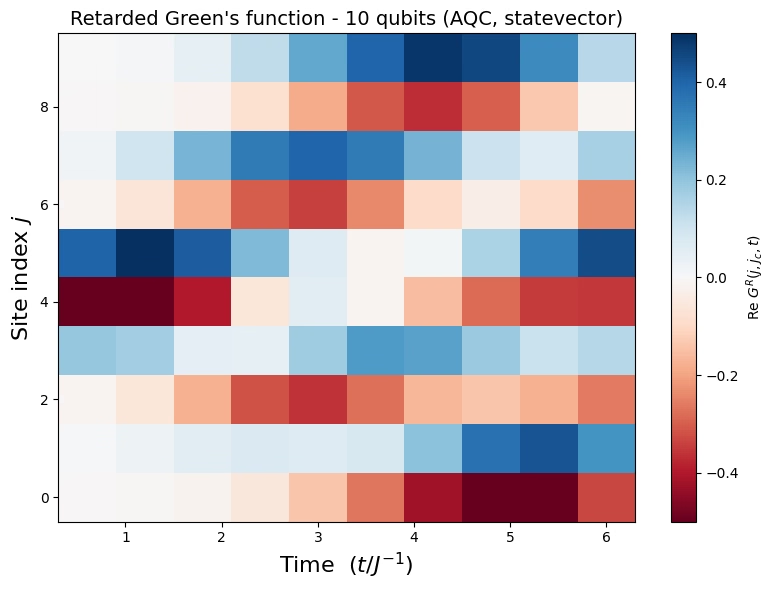
Sukatin ang per-site magnetization . Bilang function ng site at oras , ito ay eksaktong ang retarded Green's function , kaya walang kinakailangang conversion bago ang Fourier transform sa hakbang 5.
-
I-Fourier transform ang tungo sa .
Maaaring magkaroon ng mga problema sa hakbang 3, kapag ang eksaktong Trotter circuits para sa mahahabang evolution ay naging masyadong malalim para sa hardware. Tinutugunan ito ng AQC na may tensor networks sa pamamagitan ng pag-compress ng block ng Trotter steps sa isang fixed, mababaw na parameterized ansatz na ang state fidelity nito sa eksaktong evolution ay classically na-maximize gamit ang MPS simulator (arXiv:2301.08609). Ang AQC Dynamics Template ay nagpapaketa ng buong quantum core na ito (Trotter synthesis, AQC compression, at mitigated execution) sa likod ng isang tawag:
| PRE (notebook na ito) | FUNCTION (aqc-dynamics-function) | POST (notebook na ito) |
|---|---|---|
| Ground state mula sa DMRG kasama ang MPS-fidelity maximization, na may kasamang neutron kick sa parehong circuit | Trotter synthesis → AQC compression → execution sa statevector, fake, o runtime, na nagbabalik ng kada site | , ang dynamical structure factor |
Ang gawaing partikular sa eksperimento ay nananatili dito sa notebook: paghahanda ng ground-state (PRE) at ang post-processing (POST). Ang dalawang hakbang na mabigat sa quantum, ang compression at execution, ay tumatakbo sa loob ng function.
Ang tutorial na ito ay kasama ng Simulate neutron scattering in quantum materials with quantum circuits, na bumubuo ng parehong eksperimento nang inline: ang parehong KCuF na modelo, paghahanda ng ground-state, neutron kick, at post-processing, na may Trotter synthesis, AQC compression, at mitigated execution na nakasulat nang step by step. Basahin ang tutorial na iyon para malaman kung paano gumagana ang AQC compression. Basahin ang isang ito para patakbuhin ang parehong eksperimento sa pamamagitan ng isang deployed function template: ang quantum core ay naging iisang function call, at ang maraming oras na AQC compression ay tumatakbo sa loob ng Serverless worker sa halip na sa iyong makina, kaya hindi mo kailangan ng HPC system o bukas na kernel habang tumatakbo ito. Ang parehong tawag ay nagpapatakbo rin ng ibang 1D dynamics experiments.
Mga kinakailangan
Bago simulan ang tutorial na ito, tiyaking mayroon ka ng mga sumusunod:
-
Ang function na naka-deploy sa iyong Qiskit Serverless account. Patakbuhin muna ang kasamang function template: Deploy and run the AQC + Trotter dynamics function template. Gagabayan ka ng gabay na iyon sa pagkuha ng source files at pag-upload ng function sa iyong account. Ang tutorial na ito ay tumatawag lang sa naka-deploy na function.
-
Naka-save na mga kredensyal ng IBM Quantum® para sa
QiskitServerless(tingnan ang function template). Ang dalawang halimbawa sa tutorial na ito ay tumatawag sa naka-deploy na function, kaya kailangan ng parehong halimbawa ang mga ito. -
Qiskit SDK v2.0 o mas bago (
pip install qiskit). -
Ang Qiskit IBM Catalog client (
pip install qiskit-ibm-catalog). -
NumPy, SciPy, at Matplotlib (
pip install numpy scipy matplotlib). Kailangan ang SciPy 1.14 o mas bago para sa COBYQA optimizer na ginagamit sa paghahanda ng ground-state. -
Ang AQC tensor-network stack, dahil ang paghahanda ng ground-state sa Step 1 ay tumatakbo nang lokal sa notebook na ito:
pip install 'qiskit-addon-aqc-tensor[quimb-jax]==0.3.1'.
Ang unang tawag sa bagong naka-deploy na function ay naghihintay habang ini-install ng Serverless worker ang mga dependency nito, kaya asahan ang dagdag na latency sa run na iyon.
Setup
I-import ang mga library at i-define ang mga experiment-specific helper na gagamitin sa ibang pagkakataon: build_gs_ansatz (ang Hamiltonian variational ansatz, o HVA, para sa paghahanda ng ground-state), prepare_ground_state (DMRG kasama ang MPS-fidelity maximization), at get_spectrum, plot_green, at plot_spectrum (ang post-processing). Ang mga ito ay hango sa orihinal na neutron-scattering tutorial.
# Added by doQumentation — required packages for this notebook
!pip install -q matplotlib numpy qiskit qiskit-addon-aqc-tensor qiskit-ibm-catalog quimb scipy
from functools import partial

import matplotlib.pyplot as plt
import numpy as np
import scipy.optimize

import quimb.tensor as qtn
from qiskit import QuantumCircuit
from qiskit.quantum_info import SparsePauliOp
from qiskit_addon_aqc_tensor.simulation import tensornetwork_from_circuit
from qiskit_addon_aqc_tensor.simulation.quimb import QuimbSimulator
from qiskit_ibm_catalog import QiskitServerless
#  Dynamical structure factor via discrete Fourier transform

def get_spectrum(n, Gjjc, dt, time_steps, q_steps, w_steps):
    """Compute the dynamical structure factor from the retarded Green's function.

    Uses the center-site approximation and a discrete Fourier transform.
    """
    green = Gjjc / 4  # sigma -> S=1/2
    omega_max = np.pi / dt
    qpoints = np.arange(0, 2 * np.pi, 2 * np.pi / q_steps)
    omegas = np.arange(0, omega_max, omega_max / w_steps)
    green_map = np.zeros((omegas.shape[0], qpoints.shape[0]))
    center = n // 2 - 1
    for iw, w in enumerate(omegas):
        exponent = np.exp(1j * w * dt * np.arange(1, time_steps + 1))
        S_w = np.dot(green.T, exponent) * dt
        for iq, q in enumerate(qpoints):
            q_matrix = np.exp(-1j * q * np.arange(-center, center + 2, 1))
            green_map[iw, iq] = np.imag(np.dot(S_w, q_matrix))
    return green_map

#  Plotting helpers

def plot_spectrum(
    dsf,
    dt,
    q_steps,
    w_steps,
    lower_bound=False,
    upper_bound=False,
    title=None,
):
    """Heat-map of the dynamical structure factor."""
    omega_max = np.pi / dt
    qpoints = np.arange(0, 2 * np.pi, 2 * np.pi / q_steps)
    omegas = np.arange(0, omega_max, omega_max / w_steps)
    x, y = np.meshgrid(qpoints, omegas)
    fig, ax = plt.subplots(figsize=(8, 5))
    c = ax.pcolormesh(x, y, dsf / np.max(dsf), cmap="viridis", shading="auto")
    fig.colorbar(c, ax=ax, label="Normalized intensity")
    if lower_bound:
        ax.plot(
            qpoints,
            np.pi * np.abs(np.sin(qpoints)) / 2,
            "--",
            color="white",
            lw=1.5,
            label="Lower bound",
        )
    if upper_bound:
        ax.plot(
            qpoints,
            np.pi * np.abs(np.sin(qpoints / 2)),
            "--",
            color="red",
            lw=1.5,
            label="Upper bound",
        )
    ax.set_ylim(0, 3.6)
    ax.set_xlim(0, 2 * np.pi - 2 * np.pi / q_steps)
    ax.set_xlabel(r"$q$", fontsize=16)
    ax.set_ylabel(r"$\tilde{\omega} = \omega / J$", fontsize=16)
    ax.set_xticks([0, np.pi / 2, np.pi, 3 * np.pi / 2, 2 * np.pi])
    ax.set_xticklabels(["0", r"$\pi/2$", r"$\pi$", r"$3\pi/2$", r"$2\pi$"])
    if lower_bound or upper_bound:
        ax.legend(loc="upper right", fontsize=11)
    if title:
        ax.set_title(title, fontsize=14)
    plt.tight_layout()
    plt.show()

def plot_green(n, Gjjc, time_steps, dt, title=None):
    """Heat-map of the retarded Green's function in real space and time."""
    fig, ax = plt.subplots(figsize=(8, 6))
    t_axis = np.arange(1, time_steps + 1) * dt
    site_axis = np.arange(n)
    x, y = np.meshgrid(t_axis, site_axis)
    c = ax.pcolormesh(
        x,
        y,
        np.real(Gjjc).T,
        cmap="RdBu",
        vmax=0.5,
        vmin=-0.5,
        shading="auto",
    )
    fig.colorbar(c, ax=ax, label=r"Re $G^R(j, j_c, t)$")
    ax.set_xlabel(r"Time  ($t / J^{-1}$)", fontsize=16)
    ax.set_ylabel("Site index $j$", fontsize=16)
    if title:
        ax.set_title(title, fontsize=14)
    plt.tight_layout()
    plt.show()

#  Variational ground-state ansatz (HVA)

def _apply_xxz_pair_gate(qc, q0, q1, theta):
    """Apply the parameterized XXZ-type two-qubit gate used in the HVA."""
    qc.cx(q0, q1)
    qc.rz(theta, q1)
    qc.h(q0)
    qc.rz(theta + np.pi / 2, q0)
    qc.cx(q0, q1)
    qc.rz(-theta, q1)
    qc.h(q1)
    qc.cx(q1, q0)
    qc.rz(np.pi / 2, q1)
    qc.rz(-np.pi / 2, q0)
    qc.h(q1)
    qc.h(q0)

def build_gs_ansatz(n, params, layers):
    """Build the Hamiltonian variational ansatz (HVA) circuit for
    ground-state preparation of the 1D Heisenberg model.

    Starts from a product of singlet pairs and applies alternating
    odd/even layers of parameterized XXZ gates. For layer r,
    params[2 * r] is the odd-layer (inter-pair) angle and
    params[2 * r + 1] is the even-layer (intra-pair) angle.
    """
    qc = QuantumCircuit(n)
    # Initial singlet product state
    for i in range(n // 2):
        qc.x(2 * i)
        qc.x(2 * i + 1)
        qc.h(2 * i + 1)
        qc.cx(2 * i + 1, 2 * i)
    # Variational layers
    for r in range(layers):
        for i in range(1, (n + 1) // 2):  # odd layer
            _apply_xxz_pair_gate(qc, 2 * i - 1, 2 * i, params[2 * r])
        for i in range(n // 2):  # even layer
            _apply_xxz_pair_gate(qc, 2 * i, 2 * i + 1, params[2 * r + 1])
    return qc

def prepare_ground_state(n, gs_layers=5, max_bond=128, cutoff=1e-8):
    """Prepare the KCuF3 (isotropic Heisenberg) ground state as a QuantumCircuit.

    Runs DMRG (quimb MPO + DMRG2) to get the chain's ground state, then optimizes
    the HVA angles to maximize the MPS overlap |<psi_ansatz|psi_DMRG>|^2. No exact
    diagonalization, so it scales to larger n.
    """
    J = Jz = 1.0
    builder = qtn.SpinHam1D(S=1 / 2)
    builder += J * 0.5, "+", "-"
    builder += J * 0.5, "-", "+"
    builder += Jz, "Z", "Z"
    H_mpo = builder.build_mpo(L=n)
    dmrg = qtn.DMRG2(H_mpo)
    dmrg.solve(tol=1e-8, verbosity=0)

    gs_sim = QuimbSimulator(
        quimb_circuit_factory=partial(
            qtn.CircuitMPS, gate_opts=dict(cutoff=cutoff, max_bond=max_bond)
        ),
        autodiff_backend="jax",
    )

    def gs_infidelity(params):
        psi = tensornetwork_from_circuit(
            build_gs_ansatz(n, params, gs_layers), gs_sim
        ).psi
        return 1 - abs(psi.H @ dmrg.state) ** 2

    # Seed and optimizer match the original tutorial. Each layer starts at
    # [0, pi/2]: an odd-layer angle of 0 makes the inter-pair gate the identity,
    # and an even-layer angle of pi/2 makes the intra-pair gate a SWAP (since
    # 0.5 * (XX + YY + ZZ) = SWAP - I/2). That puts the seed at the singlet-pair
    # product limit, which is already a decent approximation to the Heisenberg
    # ground state, so the optimizer only has to refine it. The small jitter
    # (fixed RNG seed, so runs are reproducible) breaks the exact symmetry
    # between layers; COBYQA then runs for up to 100 iterations.
    rng = np.random.default_rng(12345)
    x0 = np.tile([0.0, np.pi / 2], gs_layers) + rng.normal(
        scale=0.1, size=2 * gs_layers
    )
    result_gs = scipy.optimize.minimize(
        gs_infidelity, x0, method="COBYQA", options={"maxiter": 100}
    )
    print(f"DMRG ground-state energy: {dmrg.energy:.6f}")
    print(f"GS fidelity: {1 - result_gs.fun:.4f}")
    return build_gs_ansatz(n, result_gs.x, gs_layers)

print("Setup complete - helpers defined.")
Setup complete - helpers defined.
I-load ang function template
Kumonekta sa Qiskit Serverless at i-load ang naka-deploy na aqc-dynamics-function. Ang dalawang halimbawa sa tutorial na ito ay tumatawag sa parehong fn handle, kaya ang function ay lino-load nang isang beses lang, dito.
# Credentials are read from the account saved once via QiskitServerless.save_account(...)
serverless = QiskitServerless()
fn = serverless.load("aqc-dynamics-function")
Halimbawa ng small-scale simulator
Una nating patatakbuhin ang buong workflow sa isang maliit na 10-site chain gamit ang eksaktong statevector backend. Vine-validate nito ang PRE → FUNCTION → POST pipeline bago gumasta ng anumang oras ng QPU.
Step 1: I-map ang classical inputs sa isang quantum problem
Bumuo ng KCuF Hamiltonian bilang SparsePauliOp (isotropic Heisenberg: sa coupling na sa bawat nearest-neighbor bond; ang mga string ay Pauli operators, kaya ang ay nagbibigay ng spin- coupling). Ihanda ang ground state gamit ang DMRG kasama ang MPS-fidelity maximization, pagkatapos ay isama ang neutron kick: isang -rotation sa gitnang site. Ang inihandang circuit ang ipinapasa natin sa function bilang initial_state. Iniiwan natin ang observables sa default nito (per-site ), na eksaktong ang readout na kailangan ng neutron workflow.
n = 10
dt = 0.6  # physical time per Trotter step (also the omega-axis unit in POST)
time_steps = 10
center = n // 2 - 1

# MPS-simulator settings, shared by the ground-state prep here and the AQC
# compression inside the function (matches the original tutorial).
mps_max_bond = 32
mps_cutoff = 1e-8

# 1D isotropic Heisenberg (KCuF3) Hamiltonian on n qubits
H = SparsePauliOp.from_sparse_list(
    [(p, [i, i + 1], 0.25) for i in range(n - 1) for p in ("XX", "YY", "ZZ")],
    num_qubits=n,
)

# Ground state (DMRG + fidelity max) + neutron kick baked into the same circuit
gs_circuit = prepare_ground_state(
    n, gs_layers=3, max_bond=mps_max_bond, cutoff=mps_cutoff
)
gs_circuit.rz(
    np.pi / 2, center
)  # exp(-i (pi/2)/2 Z_center): the neutron perturbation
print(
    f"Prepared {n}-qubit ground state with the neutron kick at site {center}."
)
DMRG ground-state energy: -4.258035
GS fidelity: 0.9841
Prepared 10-qubit ground state with the neutron kick at site 4.
Steps 2 at 3: I-compress at isagawa gamit ang function template
Sa isang manu-manong workflow, dalawang hiwalay na yugto ang mga ito: i-optimize ang mga circuit para sa hardware (Step 2) at isagawa ang mga ito (Step 3). Pinagsasama ng function template ang dalawa sa iisang tawag. Isinasagawa nito ang Trotter synthesis, AQC compression, at hardware transpilation, pagkatapos ay pinatatakbo ang mga circuit (dito sa eksaktong simulator, mamaya na may built-in error mitigation sa hardware). Ang dalawang tuning parameter ay aqc_segments (ang compression plan) at aqc_options (ang mga setting ng MPS at optimizer). Bawat segment na {"n_steps": k, "ansatz_steps": m} ay ni-i-compress ang k na magkakasunod na Trotter steps sa isang ansatz na binuo mula sa m-step na Trotter target, at anumang steps lampas sa sum(n_steps) ay tumatakbo bilang plain Trotter. Ang unang, mababa ang entanglement na mga steps ay ma-compress nang maganda sa isang mababaw (ansatz_steps=1) na ansatz, kaya dito, ni-i-compress natin ang unang tatlong steps sa isang single-layer na ansatz at ang susunod na dalawa sa isang mas malalim na two-layer na ansatz; ang natitirang lima sa 10 Trotter steps ay tumatakbo bilang plain Trotter. Para sa aqc_options, sinasalamin natin ang orihinal na tutorial: MPS bond dimension na max_bond=32, cutoff=1e-8, at isang L-BFGS-B optimizer na naka-cap sa 100 iterations.
Tawagin ang function na na-load sa Setup. Pinatatakbo ng backend="statevector" ang eksaktong reference path: walang oras ng QPU, na may mga circuit na tumatakbo sa isang eksaktong statevector simulator sa loob ng serverless worker (kailangan pa rin ng naka-save na Qiskit Serverless account para tawagin ito). Dala ng initial_state ang inihandang ground state (kasama ang kick); inaalis ang observables kaya sinusukat ng function ang default na per-site .
job = fn.run(
    t_steps=time_steps,
    aqc_segments=[
        {
            "n_steps": 3,
            "ansatz_steps": 1,
        },  # early steps -> shallow 1-layer ansatz
        {
            "n_steps": 2,
            "ansatz_steps": 2,
        },  # later steps -> deeper 2-layer ansatz
    ],
    aqc_options={
        "max_bond": mps_max_bond,  # MPS bond dimension for AQC compression
        "cutoff": mps_cutoff,
        "optimizer_settings": {
            "method": "L-BFGS-B",
            "jac": True,
            "options": {"maxiter": 100},
        },
    },
    dt=dt,
    hamiltonian=H,
    initial_state=gs_circuit,  # prepared ground state including the neutron kick
    # observables omitted -> default per-site Z (the neutron sigma_z readout)
    backend="statevector",
)
print(job.status()) # rerun this cell until status says DONE
DONE
# The per-site <sigma_z>(t) the function returns is the retarded Green's function
# G(j, j_c, t). The workflow samples t = 1..time_steps, so drop the t = 0 row (the
# prepared+kicked state before any evolution) before post-processing.
result = job.result()
print(
    "AQC fidelities:",
    {k: round(v, 4) for k, v in result["metadata"]["aqc_fidelities"].items()},
)

ev = np.array(result["expectation_values"])
Gjjc = ev[1:]  # shape (time_steps, n)
print("Green's function shape:", Gjjc.shape)
AQC fidelities: {'1': 1.0, '2': 0.9999, '3': 0.9992, '4': 0.9998, '5': 0.9995}
Green's function shape: (10, 10)
Step 4: I-post-process at ibalik ang resulta sa nais na classical format
I-Fourier-transform ang Green's function tungo sa , i-mirror-symmetrize, at i-clip ang mga negative: ang karaniwang post-processing ng neutron. Eksakto ang mirroring dahil para sa modelong ito, at ang mga negative na halaga na nananatili ay artifacts ng pag-Fourier-transform ng finite, discretely sampled na time series, kaya sila ay ni-clip sa zero. Sa maliit na eksaktong run na ito, ang two-spinon continuum ay marahang lang na-resolve, ngunit magkatulad ang mekanismo sa hardware run na susunod.
q_res, w_res = 100, 100
spectrum = get_spectrum(n, Gjjc, dt, time_steps, q_res, w_res)
spectrum = -(spectrum + spectrum[:, ::-1]) / 2  # mirror symmetry
spectrum = np.clip(spectrum, a_min=0, a_max=None)  # clip negatives

plot_green(
    n,
    Gjjc,
    time_steps,
    dt,
    title=f"Retarded Green's function - {n} qubits (AQC, statevector)",
)
plot_spectrum(
    spectrum,
    dt,
    q_res,
    w_res,
    lower_bound=True,
    upper_bound=True,
    title=f"Dynamical structure factor - {n} qubits (AQC, statevector)",
)
Halimbawa ng large-scale hardware
Ang parehong workflow ay lumalaki nang hindi binabago ang anuman sa science code: isang 30-site chain, dalawang beses ang lalim ng Trotter (20 steps), isang compression plan na nagbabago ng lalim ng ansatz (mas malalim na ansatz para sa mas huling, mas maraming entanglement na steps), at execution sa isang IBM Quantum processor gamit ang built-in error mitigation ng function (dynamical decoupling, Pauli twirling, at twirled readout error extinction (TREX)). Dadaan tayo sa parehong apat na hakbang gaya ng halimbawa ng simulator, gamit muli ang fn handle mula sa Setup.
| Maliit na sukat | Malaking sukat | |
|---|---|---|
| Qubits | 10 | 30 |
| Trotter steps | 10 | 20 |
| AQC-compressed steps (1-layer + 2-layer) | 3 + 2 = 5 | 6 + 4 = 10 |
| Ground-state ansatz layers | 3 | 5 |
| MPS max bond dimension | 32 | 128 |
| Backend | statevector | QPU na may DD, Pauli twirling, at TREX |
Step 1: I-map ang classical inputs sa isang quantum problem
Bumuo ng parehong KCuF Heisenberg SparsePauliOp at ihanda ang ground state, ngayon na may mas malalim na gs_layers=5 na ansatz para sa mas mahabang chain, pagkatapos ay isama ang na neutron kick sa gitnang site. Ito ay kapareho ng mapping ng small-scale, ngunit sa .
Asahan ang mas mababang ground-state fidelity kumpara sa 10-site run: mga 0.82 dito laban sa 0.98 para sa mas maliit na chain, dahil hindi kayang saklawin ng limang HVA layer nang buo ang isang 30-site ground state. Inaasahan ito at hindi kabiguan, at tinatanggap ng orihinal na tutorial ang mga 0.65 sa 50 sites sa parehong dahilan. Ang pagtaas ng gs_layers o ng COBYQA iteration cap ay nagpapabuti nito, sa karagdagang gastos sa klasikal na computation.
n = 30
dt = 0.6
time_steps = 20
center = n // 2 - 1

# Same MPS settings as the original large-scale run: a larger bond for the
# longer, more-entangled chain (shared by GS prep and AQC compression).
mps_max_bond = 128
mps_cutoff = 1e-8

# Same KCuF3 Hamiltonian and ground-state prep, on a larger chain
H = SparsePauliOp.from_sparse_list(
    [(p, [i, i + 1], 0.25) for i in range(n - 1) for p in ("XX", "YY", "ZZ")],
    num_qubits=n,
)
gs_circuit = prepare_ground_state(
    n, gs_layers=5, max_bond=mps_max_bond, cutoff=mps_cutoff
)
gs_circuit.rz(np.pi / 2, center)  # neutron kick at the center site
print(
    f"Prepared {n}-qubit ground state with the neutron kick at site {center}."
)
DMRG ground-state energy: -13.111355
GS fidelity: 0.8201
Prepared 30-qubit ground state with the neutron kick at site 14.
Steps 2 at 3: I-compress at patakbuhin gamit ang function template
Ang parehong iisang tawag gaya sa halimbawa ng simulator, ngayon ay may backend_name na nakaturo sa isang IBM Quantum processor, kaya doon nagta-transpile at nagpapatupad ang function. Ang compression plan ay nag-iiba-iba ng lalim ng ansatz: ang unang anim (mababang-entanglement) na Trotter step ay kino-compress sa isang mababaw na single-layer ansatz, ang susunod na apat sa mas malalim na two-layer ansatz, at ang natitirang 10 sa 20 steps ay tumatakbo bilang plain Trotter. Itinataas ng aqc_options ang MPS bond dimension sa max_bond=128 para sa mas mahaba, mas entangled na chain (kaayon ng orihinal), habang pinapanatili ang parehong L-BFGS-B optimizer na naka-cap sa 100 iterations. Ang estimator_options ay nagpapagana ng built-in na error mitigation: dynamical decoupling (XY4), gate twirling, at TREX measurement mitigation. Ang mga default ng function ay tumutugma na sa orihinal na tutorial para sa lahat ng ito maliban sa TREX learning budget (measure_noise_learning). Isinusulat pa rin ang buong block dahil pinapalitan nang buo ng caller-supplied na estimator_options ang mga default ng function sa halip na pagsamahin sa mga ito, kaya ang pagtanggal ng isang key ay babalik sa default ng IBM Quantum Compute sa halip na sa default ng function.
# Steps 2 + 3: the function compresses (varied ansatz) and executes on hardware.
job = fn.run(
    t_steps=time_steps,
    aqc_segments=[
        {
            "n_steps": 6,
            "ansatz_steps": 1,
        },  # early steps -> shallow 1-layer ansatz
        {
            "n_steps": 4,
            "ansatz_steps": 2,
        },  # later steps -> deeper 2-layer ansatz
    ],
    aqc_options={
        "max_bond": mps_max_bond,  # 128 for the longer chain
        "cutoff": mps_cutoff,
        "optimizer_settings": {
            "method": "L-BFGS-B",
            "jac": True,
            "options": {"maxiter": 100},
        },
    },
    dt=dt,
    hamiltonian=H,
    initial_state=gs_circuit,
    backend_name="ibm_pittsburgh",
    # Mitigation settings from the original tutorial. Only the two
    # measure_noise_learning values differ from the function's defaults; the rest
    # restates them, because a caller-supplied estimator_options dict replaces the
    # function's defaults wholesale rather than merging into them.
    estimator_options={
        "environment": {"job_tags": ["TUT-SNS"]},
        "dynamical_decoupling": {"enable": True, "sequence_type": "XY4"},
        "twirling": {
            "enable_gates": True,
            "num_randomizations": 1000,
            "shots_per_randomization": 128,
        },
        "resilience": {
            "measure_mitigation": True,
            "measure_noise_learning": {
                "num_randomizations": 32,
                "shots_per_randomization": 100,
            },
        },
    },
)
print("job ID (save this to reconnect later):", job.job_id)
job ID (save this to reconnect later): 43ed8d07-6d7d-4f33-b70a-7f31b765b310
Ang malakihang run ay hindi mabilis, at karamihan sa oras ay klasikal sa halip na nasa QPU. Ang AQC compression ay tumatakbo sa loob ng function bago pa man makarating ang anuman sa QPU: sa 30 sites na may max_bond=128 halos apat na oras ito sa aming run, laban sa mga 18 minuto ng QPU time na binanggit sa Usage estimate sa itaas ng tutorial na ito. Nasa ibabaw pa ng pareho ang paghihintay sa queue. Hindi mo kailangang panatilihing bukas ang notebook o kernel na ito habang tumatakbo ito.
Kopyahin ang job ID na naka-print ng nakaraang cell at i-save ito. Ang susunod na tatlong cell ay nagbibigay-daan sa iyong ipagpatuloy ang run sa ibang pagkakataon:
-
Mag-reconnect, kailangan lang sa bagong kernel session: patakbuhin muli ang mga cell sa Setup para muling likhain ang
serverless, pagkatapos ay muling itayo angjobhandle mula sa ID na na-save mo. Laktawan ang cell na ito kung nasa session ka pa rin kung saan mo isinumite ito, dahil live na ang handle. -
Suriin ang status: patakbuhin muli hanggang mag-report ito ng
DONE. -
Kunin ang resulta: patakbuhin lamang kapag ang status ay
DONE.
Ang sumusunod na reconnect cell ay may placeholder. Palitan ito ng iyong sariling job_id:
# Reconnect to a previously submitted job by its ID. Only needed in a NEW kernel
# session; if you are still in the session where you submitted, the `job` handle
# from the preceding cell is already live, so skip this cell. Replace the ID that follows with your own.
job = serverless.get_job_by_id("<your job ID>")
# Check where the job is. Re-run this until it reports DONE before fetching the
# result in the following cell: QUEUED -> INITIALIZING -> RUNNING: OPTIMIZING_FOR_HARDWARE ->
# RUNNING: WAITING_FOR_QPU -> RUNNING: EXECUTING_QPU -> RUNNING: POST_PROCESSING
# -> DONE.
print(job.status())
DONE
# Run this only once the preceding status cell reports DONE. result() blocks until
# the job finishes, so calling it earlier just waits (possibly for hours).
result = job.result()
print(
    "AQC fidelities:",
    {k: round(v, 4) for k, v in result["metadata"]["aqc_fidelities"].items()},
)

ev = np.array(result["expectation_values"])
Gjjc = ev[1:]  # drop the t = 0 row -> shape (time_steps, n)
AQC fidelities: {'1': 1.0, '2': 0.9994, '3': 0.9944, '4': 0.9853, '5': 0.9747, '6': 0.959, '7': 0.9495, '8': 0.9542, '9': 0.9533, '10': 0.9451}
Step 4: I-post-process at ibalik ang resulta sa nais na classical format
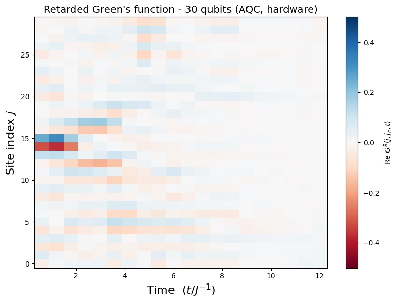
Kapareho ang post-processing sa simulator run: i-Fourier-transform ang Green's function sa , i-mirror-symmetrize, at putulin ang mga negatibo. Sa mas mahabang chain at ebolusyon, mas malinaw na nareresolba ang two-spinon continuum. Dapat pumuno ito sa band sa pagitan ng mga dashed bound, pinakamaliwanag malapit sa .
n = result["metadata"]["n"]
q_res, w_res = 100, 100
spectrum = get_spectrum(n, Gjjc, dt, time_steps, q_res, w_res)
spectrum = -(spectrum + spectrum[:, ::-1]) / 2  # mirror symmetry
spectrum = np.clip(spectrum, a_min=0, a_max=None)  # clip negatives

plot_green(
    n,
    Gjjc,
    time_steps,
    dt,
    title=f"Retarded Green's function - {n} qubits (AQC, hardware)",
)
plot_spectrum(
    spectrum,
    dt,
    q_res,
    w_res,
    lower_bound=True,
    upper_bound=True,
    title=f"Dynamical structure factor - {n} qubits (AQC, hardware)",
)
Appendix
Ang naunang hardware example ay nagpapatakbo ng iisang haba ng chain. Ang tatlong spectra na sumusunod ay mula sa mga naunang hardware run ng parehong workflow na ito sa ibm_pittsburgh sa 10, 20, at 30 sites, kung saan pinananatiling fixed ang bawat ibang input: 20 Trotter steps sa dt = 0.6, ang compression plan na anim na one-layer kasama ang apat na two-layer na AQC-compressed steps, at max_bond = 128. Ito ay mga naitalang resulta, hindi output mula sa mga naunang cell.
Ginagamit ang parehong mga setting sa lahat ng tatlong sukat, kaya direktang maihahambing ang mga spectra. Ang pag-tune sa mga ito ayon sa haba ng chain, halimbawa may higit pang ground-state ansatz layers o mas malaking max_bond, ay maaaring magbigay ng mas mahusay na resulta kaysa sa anumang ipinakita rito.
Mga susunod na hakbang
-
I-adapt ang workflow na ito sa iyong sariling sistema: tinatanggap ng function ang anumang 1D nearest-neighbor na
SparsePauliOp, kaya't ang ibang chain Hamiltonian, initial state, o set ng observables ay tumatakbo sa parehong PRE → FUNCTION → POST pipeline. Tingnan ang buong input/output contract sa AQC Dynamics Template sa GitHub. -
Basahin ang papel kung saan nanggaling ang benchmark na ito: Lee et al., Benchmarking quantum simulation with neutron-scattering experiments (arXiv:2603.15608).
-
Ikumpara sa orihinal na "Simulate neutron scattering" tutorial, ang inline workflow na ini-port ng tutorial na ito papunta sa isang deployed function template.
-
Alamin pa ang tungkol sa mga error mitigation at suppression techniques na inilapat sa hardware run: dynamical decoupling, Pauli twirling, at TREX.