Quantum approximate multi-objective optimization
Tantiya sa paggamit: 10 minuto sa isang Heron r2 processor (TANDAAN: Tantiya lang ito. Maaaring iba ang runtime mo.)
Mga learning outcome
Nilulutas ng tutorial na ito ang isang cardinality-constrained na problema sa portfolio optimization: dahil sa constraint na humawak ng eksaktong asset, balansehin ang mga layunin sa risk, return, at diversification para mahanap ang hanay ng mga optimal na portfolio.
Pagkatapos makumpleto ang tutorial na ito, maaasahan mong maiintindihan mo ang:
-
Paano ipahayag ang isang problema sa pagpili ng portfolio na may tatlong magkakalabang layunin — mababang risk, mataas na return, at mahusay na diversification — bilang isang quantum optimization problem.
-
Paano ang isang QAOA circuit, na iniikot sa isang hanay ng mga objective weight, ay gumuguhit ng Pareto front ng mga optimal na trade-off na portfolio.
-
Paano pinananatili ng isang XY mixer ang paghahanap sa loob ng subspace na "pumili ng eksaktong K asset", kaya hindi na kailangan ng penalty term at ipinapatupad ang feasibility sa pamamagitan ng post-selection ng mga nasukat na bitstring.
-
Paano sanayin ang mga angle ng circuit gamit ang matrix-product-state simulator sa sukat na masyadong malaki para i-optimize nang eksakto, kasunod ng Kotil et al. (arXiv:2503.22797).
Mga paunang kinakailangan
Inirerekomendang pamilyar ka sa:
-
Ang workflow ng Qiskit patterns (map, optimize, execute, post-process).
-
Ang mga batayan ng QAOA.
Background
Bihirang nag-o-optimize ang isang portfolio manager ng iisang numero. Gusto nilang mataas ang mga return, mababa ang risk (ang variance ng mga return na iyon), at nakakalat ang mga hawak sa iba't ibang sector para hindi sobrang nakalantad ang portfolio sa iisang bahagi ng merkado. Nagbabanggaan ang mga layuning ito: ang mga asset na may pinakamataas na return ay madalas ang pinakamaligalig, at ang pagtutok sa isang hot na sector ay nakakasama sa diversification.
Walang iisang "pinakamahusay" na portfolio. Sa halip, may Pareto front: ang hanay ng mga portfolio kung saan hindi mo mapapabuti ang isang layunin nang hindi isinusuko ang isa pa. Layunin nating iguhit ang front na iyon para makapili ang gagawa ng desisyon ng trade-off na gusto niya.
Inilalatag natin ang problema bilang pagpili ng eksaktong asset mula sa (ang bawat asset ay kasama o hindi — isang qubit bawat asset). Tatlong Hamiltonian ang nag-e-encode ng tatlong layunin. Pinagsasama natin ang mga ito gamit ang mga weight na na nasa isang simplex (ang kabuuan ay isa), at ang isang QAOA sampler ay nagbabalik ng magagandang portfolio para sa bawat pagpili ng weight. Ang pag-ikot sa mga weight ay nag-iikot sa relatibong kahalagahan ng risk laban sa return laban sa diversification, at ang union ng lahat ng na-sample na portfolio ay gumuguhit ng Pareto front.
Una nating tatalakayin ang buong workflow sa isang maliit na halimbawang may walong asset na mabe-verify natin sa brute force, at pagkatapos ay patatakbuhin ang parehong pamamaraan sa isang 40-asset na instance na angkop sa quantum hardware.
Itinuturo ng tutorial na ito ang workflow (mapping, angle training, constrained sampling, at Pareto post-processing), sa halip na ipakita ang quantum advantage. Sa sukat na 40 asset na ginamit dito, halos kasing-husay ng QAOA sampler ang uniform random sampling, at tahasan naming ipinapakita ang paghahambing na iyon.
Mga kinakailangan
Bago simulan ang tutorial na ito, tiyaking naka-install ang mga sumusunod:
-
Qiskit SDK v2.0 o mas bago, na may suporta sa visualization
-
Qiskit Runtime v0.22 o mas bago (
pip install qiskit-ibm-runtime) -
Qiskit Aer (
pip install qiskit-aer) -
Ang Optimization mapper Qiskit addon (
pip install qiskit-addon-opt-mapper) at ang QAOA training pipeline, naka-pin sav0.1.0tag:pip install "git+https://github.com/qiskit-community/qaoa_training_pipeline.git@v0.1.0" -
moocorepara sa mga kalkulasyon ng Pareto-front at hypervolume (pip install moocore)
Setup
I-import ang mga library na ginagamit sa buong tutorial at magtakda ng random seed para sa reproducibility.
# Added by doQumentation — installs the packages this notebook needs if they are missing
import importlib.util

_needed = {"matplotlib": "matplotlib", "moocore": "moocore", "numpy": "numpy", "qaoa_training_pipeline": "git+https://github.com/qiskit-community/qaoa_training_pipeline.git@v0.1.0", "qiskit": "qiskit", "qiskit_addon_opt_mapper": "qiskit-addon-opt-mapper", "qiskit_aer": "qiskit-aer", "qiskit_ibm_runtime": "qiskit-ibm-runtime", "scipy": "scipy"}
_missing = [pip for module, pip in _needed.items()
            if importlib.util.find_spec(module) is None]
# One at a time, so a package that fails to install does not block the others
for _pip in _missing:
    %pip install -q {_pip}
if not _missing:
    print("\u2713 All required packages are installed")
import numpy as np
import matplotlib.pyplot as plt
from math import comb
from moocore import hypervolume, filter_dominated, is_nondominated

from qiskit import QuantumCircuit
from qiskit.circuit import ParameterVector
from qiskit.circuit.library import qaoa_ansatz
from qiskit.quantum_info import SparsePauliOp
from qiskit.transpiler import generate_preset_pass_manager
from qiskit_aer.primitives import SamplerV2 as AerSampler
from qiskit_addon_opt_mapper.problems import OptimizationProblem
from qaoa_training_pipeline.training import ScipyTrainer
from qaoa_training_pipeline.evaluation import (
    StatevectorEvaluator,
    MPSAerEvaluator,
)

np.random.seed(42)
sampler = AerSampler(seed=42)  # local simulator for the small-scale example
print("Setup complete.")
Setup complete.
Halimbawa sa maliit na sukat gamit ang simulator
Magsisimula tayo sa walong asset mula sa anim na sector at pipili ng eksaktong sa mga ito. Sa walong asset lang, mayroon lang na valid na portfolio, kaya masusuri natin mamaya ang quantum na resulta laban sa exhaustive search.
Hakbang 1: I-map ang mga classical na input sa isang quantum na problema
Ang bawat asset ay isang qubit; ang bitstring na gaya ng 10110010 ay isang portfolio (ang mga 1 ay ang mga asset na hawak natin). Kailangan natin ng tatlong sangkap: ang market data, ang tatlong objective Hamiltonian, at isang circuit na nagmumungkahi lang ng mga portfolio na may eksaktong asset.
# --- Small-scale universe: 8 assets across 6 sectors ---
tickers = ["AAPL", "XOM", "JPM", "JNJ", "KO", "AMT", "AMZN", "SLB"]
sectors = [
    "Tech",
    "Energy",
    "Finance",
    "Health",
    "Staples",
    "REIT",
    "Tech",
    "Energy",
]
n_assets = len(tickers)
K = 4  # choose exactly K assets
n_obj = 3  # risk, return, diversification

# Annualized expected returns
mu = np.array([0.28, 0.12, 0.22, 0.05, 0.08, 0.10, 0.32, 0.15])

# Annualized covariance matrix (the "risk" model)
sigma = np.array(
    [
        [0.070, 0.010, 0.020, 0.008, 0.005, 0.012, 0.045, 0.011],
        [0.010, 0.065, 0.015, 0.006, 0.004, 0.008, 0.009, 0.050],
        [0.020, 0.015, 0.055, 0.010, 0.007, 0.015, 0.018, 0.014],
        [0.008, 0.006, 0.010, 0.030, 0.012, 0.009, 0.007, 0.005],
        [0.005, 0.004, 0.007, 0.012, 0.025, 0.006, 0.004, 0.003],
        [0.012, 0.008, 0.015, 0.009, 0.006, 0.045, 0.011, 0.007],
        [0.045, 0.009, 0.018, 0.007, 0.004, 0.011, 0.085, 0.010],
        [0.011, 0.050, 0.014, 0.005, 0.003, 0.007, 0.010, 0.072],
    ]
)

# Diversification score: number of cross-sector pairs in the portfolio.
# D[i,j] = 0.5 when assets i and j are in different sectors, so x^T D x counts
# the cross-sector pairs. More cross-sector pairs = better diversified.
D = np.array(
    [
        [1.0 if sectors[i] != sectors[j] else 0.0 for j in range(n_assets)]
        for i in range(n_assets)
    ]
)
np.fill_diagonal(D, 0.0)
D = D / 2

print(f"{n_assets} assets, choose K={K}, {n_obj} objectives")
for t, s, m in zip(tickers, sectors, mu):
    print(f"  {t:5s} ({s:8s})  expected return {m:5.0%}")
8 assets, choose K=4, 3 objectives
  AAPL  (Tech    )  expected return   28%
  XOM   (Energy  )  expected return   12%
  JPM   (Finance )  expected return   22%
  JNJ   (Health  )  expected return    5%
  KO    (Staples )  expected return    8%
  AMT   (REIT    )  expected return   10%
  AMZN  (Tech    )  expected return   32%
  SLB   (Energy  )  expected return   15%
# Each objective becomes a Hamiltonian whose lowest-energy bitstrings are the
# best portfolios for that objective. The opt-mapper turns a plain
# min/max problem over binary variables into the equivalent Ising operator.
def build_risk_hamiltonian(sigma, n):
    """Minimize portfolio variance x^T sigma x  (quadratic -> ZZ terms)."""
    prob = OptimizationProblem("risk")
    prob.binary_var_list(n)
    prob.minimize(quadratic=sigma)
    op, _ = prob.to_ising()
    return op.simplify()

def build_return_hamiltonian(mu, n):
    """Maximize expected return mu . x  (linear -> Z terms)."""
    prob = OptimizationProblem("return")
    prob.binary_var_list(n)
    prob.maximize(linear=mu)
    op, _ = prob.to_ising()
    return op.simplify()

def build_diversity_hamiltonian(D, n):
    """Maximize cross-sector pairs x^T D x  (quadratic -> ZZ terms)."""
    prob = OptimizationProblem("diversity")
    prob.binary_var_list(n)
    prob.maximize(quadratic=D)
    op, _ = prob.to_ising()
    return op.simplify()

H_risk = build_risk_hamiltonian(sigma, n_assets)
H_return = build_return_hamiltonian(mu, n_assets)
H_diversity = build_diversity_hamiltonian(D, n_assets)
cost_ops = [H_risk, H_return, H_diversity]

for name, op in zip(["risk", "return", "diversity"], cost_ops):
    print(f"H_{name:10s}: {op.size} Pauli terms")
H_risk      : 36 Pauli terms
H_return    : 8 Pauli terms
H_diversity : 34 Pauli terms
Pagpapatupad ng "eksaktong K asset" nang walang penalty. Karaniwang paraan ang magdagdag ng penalty term na pumaparusa sa mga portfolio na mali ang laki, ngunit iniuugnay nito ang bawat qubit sa bawat isa pang qubit, na humahantong sa mas malalalim na circuit pagkatapos ng transpilation. Sa halip, gumagamit tayo ng XY mixer, na naglilipat lang sa QAOA state sa pagitan ng mga bitstring na may parehong Hamming weight. Kung magsisimula tayo sa state na mayroon nang napiling asset, ang bawat portfolio na sinusuri ng circuit ay mayroon ding eksaktong asset. Ang constraint ay nakapaloob sa estruktura ng circuit sa halip na ipinapatupad ng penalty term.
Inihahanda natin nang mura ang panimulang state: i-rotate ang bawat qubit para ito ay "on" na may probability na . Kapag nilimitahan sa mga outcome na may asset, nirereproduce nito ang ideal na equal-weight (Dicke) state, kaya itinatago na lang natin ang mga nasukat na bitstring na may eksaktong na 1 — isang hakbang na tinatawag na post-selection.
def xy_mixer(n):
    """Line XY mixer: couples neighboring qubits with XX+YY. Conserves the number
    of selected assets (Hamming weight), so cardinality is preserved automatically.
    Using a line (not a full ring) keeps the circuit shallow and hardware-friendly."""
    terms = [
        (pauli, [i, i + 1], 1) for i in range(n - 1) for pauli in ("XX", "YY")
    ]
    return SparsePauliOp.from_sparse_list(terms, n)

def product_init(n, k):
    """Cheap initial state: each qubit rotated so P(selected) = k/n. Zero two-qubit
    gates. Post-selecting its weight-k outcomes reproduces the ideal Dicke state."""
    qc = QuantumCircuit(n)
    theta = 2 * np.arcsin(np.sqrt(k / n))
    for q in range(n):
        qc.ry(theta, q)
    return qc

# Combine the three objectives with weights c (bound later, at sampling time).
p_layers = 1
c = ParameterVector("c", n_obj)
# Negate the objective so the sampling phase separator matches the sign the angles
# were trained under (the trainer maximizes the negated sum); binding below keeps +gamma.
combined_cost_op = sum(
    -c[k] * H_k for k, H_k in enumerate(cost_ops)
).simplify()

ansatz = qaoa_ansatz(
    combined_cost_op,
    reps=p_layers,
    initial_state=product_init(n_assets, K),
    mixer_operator=xy_mixer(n_assets),
)
ansatz.measure_all()

betas = [p for p in ansatz.parameters if p.name.startswith("β")]
gammas = [p for p in ansatz.parameters if p.name.startswith("γ")]
print(f"Qubits: {ansatz.num_qubits} | QAOA layers: {p_layers}")
print(
    f"Tunable angles: {len(betas)} beta + {len(gammas)} gamma, plus {n_obj} objective weights"
)
Qubits: 8 | QAOA layers: 1
Tunable angles: 1 beta + 1 gamma, plus 3 objective weights
Hakbang 2: I-optimize ang problema para sa pagpapatakbo sa quantum hardware
Bago patakbuhin, ang abstract na circuit ay tina-transpile sa mga hardware-native na gate. Sa maliit na sukat na ito, sinisilip lang natin ang gastos: gaano kalalim ang circuit at ilang two-qubit gate ang ginagamit nito? (Ang mga two-qubit gate ang pangunahing pinagmumulan ng noise sa mga totoong device.)
# Bind dummy angle values so we can transpile and measure the circuit's size.
dummy = {p: 0.1 for p in ansatz.parameters}
test_pm = generate_preset_pass_manager(optimization_level=1)
test_qc = test_pm.run(ansatz.assign_parameters(dummy))

print(f"Circuit depth          : {test_qc.depth()}")
print(
    f"Two-qubit gate depth   : {test_qc.depth(lambda x: len(x.qubits) > 1)}"
)
print(f"Two-qubit gate count   : {test_qc.num_nonlocal_gates()}")
Circuit depth          : 25
Two-qubit gate depth   : 23
Two-qubit gate count   : 42
Hakbang 3: Patakbuhin gamit ang mga Qiskit primitive
Dalawang yugto. Una, sinasanay natin ang mga QAOA angle nang isang beses, gamit ang pantay na objective weight, sa isang exact statevector simulator para mahanap ang magagandang halaga ng . Pagkatapos, iniikot natin ang maraming weight vector sa simplex at sina-sample ang circuit sa bawat isa, na nangongolekta ng mga kandidatong portfolio. Dahil ang mga objective weight lang ang nagbabago sa pagitan ng mga sweep (hindi ang mga sinanay na angle), lahat ng weight vector ay isinusumite sa iisang batched na job.
# Train the angles with equal objective weights.
# The trainer maximizes energy, so we negate the (to-be-minimized) objective sum.
training_op = sum(-1.0 / n_obj * H_k for H_k in cost_ops).simplify()

# Linear-ramp initialization (Sack and Serbyn, arXiv:2101.05742)
dt = 0.75
grid = np.arange(1, p_layers + 1) - 0.5
init_params = np.concatenate((1 - grid * dt / p_layers, grid * dt / p_layers))

trainer = ScipyTrainer(
    StatevectorEvaluator(), minimize_args={"options": {"maxiter": 300}}
)
print("Training QAOA angles (exact statevector)...")
result_train = trainer.train(
    cost_op=training_op,
    mixer=xy_mixer(n_assets),
    initial_state=product_init(n_assets, K),
    params0=init_params,
)
opt = result_train["optimized_params"]
opt_betas, opt_gammas = opt[:p_layers], opt[p_layers:]
print(f"Trained beta : {opt_betas}")
print(f"Trained gamma: {opt_gammas}")
Training QAOA angles (exact statevector)...
Trained beta : [3.329186967386619]
Trained gamma: [3.4449804324291033]
def random_uniform_simplex(n_samples, n_obj=3):
    """n_samples weight vectors spread uniformly over the (n_obj-1)-simplex."""
    s = np.zeros((n_samples, n_obj + 1))
    s[:, 1:-1] = np.random.rand(n_samples, n_obj - 1)
    s[:, -1] = 1
    s = np.sort(s, axis=1)
    return np.diff(s, axis=1)

# Bind the trained angles, leaving the objective weights c free for the sweep.
param_map = {betas[i]: opt_betas[i] for i in range(p_layers)}
param_map.update({gammas[i]: opt_gammas[i] for i in range(p_layers)})
ansatz_bound = ansatz.assign_parameters(param_map)

n_samples, shots = 200, 500
c_vecs = random_uniform_simplex(n_samples, n_obj)

print(f"Sampling {n_samples} weight vectors x {shots} shots...")
result = sampler.run([(ansatz_bound, c_vecs)], shots=shots).result()

# Collect every distinct bitstring seen across all weight vectors.
all_bitstrings = set()
for s in range(n_samples):
    for bs in result[0].data.meas.get_counts(s):
        # get_counts is little-endian; reverse so bit i = asset i
        all_bitstrings.add(bs.replace(" ", "")[::-1])
print(f"Distinct portfolios sampled: {len(all_bitstrings)}")
Sampling 200 weight vectors x 500 shots...
Distinct portfolios sampled: 256
Hakbang 4: I-post-process at ibalik ang resulta sa nais na classical na format
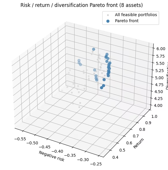
Itinatago lang natin ang mga feasible na portfolio (eksaktong asset mula sa post-selection step), binibigyan ng score ang bawat isa sa lahat ng tatlong layunin, at kinukuha ang Pareto front: ang mga portfolio na hindi natatalo sa lahat ng layunin nang sabay. Ang hypervolume ay isang numerong nagbubuod kung gaano karaming objective space ang dinodomina ng front, at mas malaki ay mas mabuti.
Sa 100,000 shot sa 256 na bitstring lang, nakikita ng run na ito ang bawat isa sa 70 valid na portfolio, kaya sa laking ito ay isa itong epektibong brute-force na pagsusuri na tama ang pagkakakabit ng pipeline, at hindi ebidensya na nahanap ng QAOA ang front.
def evaluate_portfolio(bitstring, sigma, mu, D):
    """Score one portfolio on all three objectives (all framed as 'bigger is better')."""
    x = np.array([int(b) for b in bitstring])
    # negative risk, return, diversification (cross-sector pairs)
    return np.array([-(x @ sigma @ x), x @ mu, x @ D @ x])

# Post-select feasible portfolios, then score them.
feasible = [bs for bs in all_bitstrings if bs.count("1") == K]
fis = np.array([evaluate_portfolio(bs, sigma, mu, D) for bs in feasible])

pareto_front = filter_dominated(fis, maximise=True)
ref_point = fis.min(axis=0)
qmoo_hv = hypervolume(fis, ref=ref_point, maximise=True)

print(
    f"Feasible portfolios found : {len(feasible)} of {comb(n_assets, K)} possible"
)
print(f"Pareto-front portfolios   : {len(pareto_front)}")
print(f"Hypervolume               : {qmoo_hv:.4f}")
Feasible portfolios found : 70 of 70 possible
Pareto-front portfolios   : 26
Hypervolume               : 0.2487
fig = plt.figure(figsize=(8, 6))
ax = fig.add_subplot(111, projection="3d")
ax.scatter(
    fis[:, 0],
    fis[:, 1],
    fis[:, 2],
    c="lightgray",
    s=12,
    label="All feasible portfolios",
)
ax.scatter(
    pareto_front[:, 0],
    pareto_front[:, 1],
    pareto_front[:, 2],
    c="steelblue",
    s=45,
    label="Pareto front",
)
ax.set_xlabel("Negative risk")
ax.set_ylabel("Return")
ax.set_zlabel("Diversification")
ax.set_title("Risk / return / diversification Pareto front (8 assets)")
ax.legend()
plt.tight_layout()
plt.show()
Halimbawa sa hardware sa malaking sukat
Ngayon ay ang parehong workflow sa 40 asset (8 sector × 5), na pumipili ng . Ang apatnapung qubit ay masyadong malaki para i-simulate nang eksakto (isang statevector na may amplitude), kaya hindi maaaring i-optimize ang mga angle gaya ng ginawa sa walong asset, at ang isang dense na circuit ay masyadong malalim para sa kasalukuyang hardware. Ang M na valid na portfolio ay sapat pa ring kaunti para bilangin nang classical, na ginagamit natin sa dulo bilang exact na benchmark. Maraming bagay ang nagbabago, at walang iba pang nagbabago sa pamamaraan:
-
Sanayin ang mga angle gamit ang matrix-product-state (MPS) simulator, hindi exact statevector. Alinsunod sa reference (Kotil et al.), itinatakda natin ang mga objective weight sa pantay na halaga, ino-optimize ang iisang β, γ sa MPS simulator, at ginagamit muli ang mga ito sa bawat weighting vector sa sweep. (Sinasanay natin sa laking pinapatakbo natin — walang small-to-large na angle transfer.)
-
I-sparsify ang risk model para magkasya sa hardware. Ang buong covariance ay nag-uugnay sa lahat ng 780 pares ng asset. Itinatago lang natin ang pinakamalalakas at pinakamurang i-route na mga coupling gamit ang importance-aware QAP truncation, at iniuugnay ang bawat sector sa isang magaan na ring para sa diversity term. Pinananatili nitong makabuluhan ang mga layunin habang hawak ang circuit sa laking angkop sa hardware.
-
Panatilihing mababaw ang circuit at magbigay ng tapat na score. Stochastic ang routing, kaya nagta-transpile tayo gamit ang ilang seed at itinatago ang pinakamababaw (at walang quantum time na nauubos). Ang mga portfolio ay palaging sinusukat laban sa totoo at buong mga layunin. Ang sparsification ay humuhubog lang sa circuit, hindi sa paraan ng paghusga sa mga portfolio.
Ang pagtatago lang ng pinakamalalaking coupling ng bawat asset batay sa magnitude ay maaaring magresulta sa circuit na sparse ngunit mahirap pa ring i-route. Sa halip, itinatago ng QAP truncation ang mga coupling na parehong malaki at pisikal na malapit sa chip, kaya ang parehong gate budget ay nagbibigay ng mas mababaw at mas hardware-friendly na circuit.
Hakbang 1: I-map ang mga input (na-sparsify para sa hardware)
import csv
import urllib.request

# Download the committed market-data snapshot from the repo.
# --- 40-asset universe: 8 GICS sectors x 5 tickers (real market data) ---
# Load the committed market-data snapshot (real annualized returns and covariance).
# Values are stored at the precision used to train the shipped QAOA angles
# (mu: 3 dp, sigma: 4 dp), so the pre-trained parameters in instances/ stay exactly valid.

url = "https://raw.githubusercontent.com/Qiskit/documentation/main/datasets/tutorials/qmoo/market_data.csv"
urllib.request.urlretrieve(url, "market_data.csv")

with open("market_data.csv", newline="") as _f:
    _rows = list(csv.reader(_f))

# Covariance column order
_tickers_csv = _rows[0][2:]
# Asset tickers
tickers_40 = [r[0] for r in _rows[1:]]
# Annualized expected returns
mu_40 = np.array([float(r[1]) for r in _rows[1:]])
# Covariance (risk model)
sigma_40 = np.array([[float(v) for v in r[2:]] for r in _rows[1:]])

sectors_40 = [
    "Tech",
    "Tech",
    "Tech",
    "Tech",
    "Tech",
    "Energy",
    "Energy",
    "Energy",
    "Energy",
    "Energy",
    "Finance",
    "Finance",
    "Finance",
    "Finance",
    "Finance",
    "Health",
    "Health",
    "Health",
    "Health",
    "Health",
    "Staples",
    "Staples",
    "Staples",
    "Staples",
    "Staples",
    "Industrials",
    "Industrials",
    "Industrials",
    "Industrials",
    "Industrials",
    "Utilities",
    "Utilities",
    "Utilities",
    "Utilities",
    "Utilities",
    "REIT",
    "REIT",
    "REIT",
    "REIT",
    "REIT",
]
n_assets_40 = len(tickers_40)
K_40 = 6  # choose exactly K assets

sector_names_40 = list(dict.fromkeys(sectors_40))
sect_idx_40 = np.array([sector_names_40.index(s) for s in sectors_40])
# True cross-sector diversification matrix (used for scoring)
D_40 = np.array(
    [
        [
            0.5 if sectors_40[i] != sectors_40[j] else 0.0
            for j in range(n_assets_40)
        ]
        for i in range(n_assets_40)
    ]
)
np.fill_diagonal(D_40, 0.0)
print(
    f"{n_assets_40} assets, {len(sector_names_40)} sectors, choose K={K_40}"
)
40 assets, 8 sectors, choose K=6
# Sparsify the covariance so the risk circuit fits on hardware. A small diagonal
# shift (added after truncation) keeps the risk model positive semidefinite; at fixed
# K it adds the same constant to every portfolio, so it never changes the ranking.
# Importance-aware QAP truncation (Kotil et al. style): place the qubits on a line
# and use a Quadratic Assignment Problem to choose the layout that keeps the
# strongest covariance couplings within routing distance k of the swap network,
# then drop the rest. Unlike a fixed top-k cap, it keeps couplings that are both
# large AND cheap to route.
from scipy.optimize import quadratic_assignment as qap
from qiskit.transpiler.passes.routing.commuting_2q_gate_routing import (
    SwapStrategy,
)

# Truncation level: larger k keeps more couplings (deeper circuit)
k_truncate = 2
_dist = np.array(
    SwapStrategy.from_line(list(range(n_assets_40))).distance_matrix
)

def qap_truncate(Q, k):
    w = np.abs(Q.copy())
    np.fill_diagonal(w, 0.0)
    mask = (_dist <= k).astype(float)
    # Seed the QAP solver explicitly (by default it draws from NumPy's global
    # RNG, which SciPy is deprecating) so the truncation is reproducible.
    perm = qap(-w, mask, options={"rng": np.random.default_rng(42)}).col_ind
    keep = mask[np.ix_(perm, perm)]
    Qt = Q * keep
    np.fill_diagonal(Qt, np.diag(Q))
    return Qt

sigma_sparse = qap_truncate(sigma_40, k_truncate)
print(
    f"QAP truncation (k={k_truncate}): risk edges kept = "
    f"{(np.count_nonzero(sigma_sparse) - n_assets_40) // 2}"
)
ridge = max(0.0, -np.linalg.eigvalsh(sigma_sparse)[0]) + 1e-6
sigma_sparse = sigma_sparse + ridge * np.eye(n_assets_40)

# Diversity: couple each sector's assets in a ring (sparse stand-in for the
# same-sector pair count). Scoring still uses the true cross-sector matrix D_40.
def build_same_sector_hamiltonian(D_same, n):
    prob = OptimizationProblem("diversity_sparse")
    prob.binary_var_list(n)
    prob.minimize(quadratic=D_same)
    op, _ = prob.to_ising()
    return op.simplify()

D_ring = np.zeros((n_assets_40, n_assets_40))
for s in set(sect_idx_40):
    members = np.where(sect_idx_40 == s)[0]
    for k in range(len(members)):
        i, j = members[k], members[(k + 1) % len(members)]
        D_ring[i, j] = D_ring[j, i] = 0.5

H_risk_40 = build_risk_hamiltonian(sigma_sparse, n_assets_40)
H_return_40 = build_return_hamiltonian(mu_40, n_assets_40)
H_diversity_40 = build_same_sector_hamiltonian(D_ring, n_assets_40)
cost_ops_40 = [H_risk_40, H_return_40, H_diversity_40]
n_zz = sum(
    1 for p in sum(cost_ops_40).simplify().paulis if str(p).count("Z") == 2
)
print(
    f"Cost-layer interactions: {n_zz} (dense would be {n_assets_40*(n_assets_40-1)//2})"
)
QAP truncation (k=2): risk edges kept = 78
Cost-layer interactions: 102 (dense would be 780)
Mga Hakbang 2-3: sanayin ang mga angle, pagkatapos ay buuin at isumite ang hardware job
Ang apatnapung qubit ay masyadong malaki para i-optimize nang eksakto ang mga angle, kaya sinasanay natin ang iisang sa isang matrix-product-state simulator sa pantay na objective weight at ginagamit muli ang mga ito sa buong sweep. Ang cell sa ibaba ay naglo-load ng mga pre-trained na halaga mula sa isang file. Maliit ang sinanay na cost-layer angle (), kaya ang circuit ay naglalapat ng banayad na bias sa halip na matalas na projection.
import json
from qiskit_ibm_runtime import QiskitRuntimeService, SamplerV2

# Pre-trained angles loaded from a file (training is slow; QDC pattern).
# Set load_params_file = False to retrain in-notebook.
load_params_file = True
params_url = "https://raw.githubusercontent.com/Qiskit/documentation/main/datasets/tutorials/qmoo/qaoa_params.json"
params_path = "qaoa_params.json"
if load_params_file:
    urllib.request.urlretrieve(params_url, params_path)
    qaoa_params = json.load(open(params_path))
    p_layers_hw = qaoa_params["p_layers"]
    opt_betas_40, opt_gammas_40 = qaoa_params["betas"], qaoa_params["gammas"]
else:
    # Same workflow as the small-scale example: qaoa_training_pipeline's MPSAerEvaluator
    # evaluates the QAOA energy on Aer's MPS simulator and supports the XY mixer.
    # As in the small-scale example the trainer maximizes energy, so we negate the
    # (to-be-minimized) objective sum; the 1/n_obj scaling matches the equal-weight
    # point of the sweep, so the trained gamma transfers directly to the weighted circuits.
    p_layers_hw = 1
    training_op_40 = sum(-1.0 / n_obj * H_k for H_k in cost_ops_40).simplify()

    dt = 0.75
    grid = np.arange(1, p_layers_hw + 1) - 0.5
    init_params_40 = np.concatenate(
        (1 - grid * dt / p_layers_hw, grid * dt / p_layers_hw)
    )

    trainer_40 = ScipyTrainer(
        MPSAerEvaluator({"matrix_product_state_max_bond_dimension": 24}),
        minimize_args={"options": {"maxiter": 80}},
    )
    print("Training QAOA angles (MPS simulator)...")
    result_train_40 = trainer_40.train(
        cost_op=training_op_40,
        mixer=xy_mixer(n_assets_40),
        initial_state=product_init(n_assets_40, K_40),
        params0=init_params_40,
    )
    opt_40 = result_train_40["optimized_params"]
    opt_betas_40, opt_gammas_40 = (
        list(opt_40[:p_layers_hw]),
        list(opt_40[p_layers_hw:]),
    )
    import os

    os.makedirs(os.path.dirname(params_path) or ".", exist_ok=True)
    json.dump(
        {
            "p_layers": p_layers_hw,
            "betas": opt_betas_40,
            "gammas": opt_gammas_40,
        },
        open(params_path, "w"),
        indent=2,
    )
    print(
        f"Trained angles saved to {params_path} (set load_params_file=True to reuse)."
    )

c40 = ParameterVector("c", n_obj)
# Negated to match the trained angles' sign, as in the small-scale cell; binding keeps +gamma.
combined_cost_op_40 = sum(
    -c40[k] * H_k for k, H_k in enumerate(cost_ops_40)
).simplify()
qc_40 = qaoa_ansatz(
    combined_cost_op_40,
    reps=p_layers_hw,
    initial_state=product_init(n_assets_40, K_40),
    mixer_operator=xy_mixer(n_assets_40),
)
qc_40.measure_all()
b40 = [p for p in qc_40.parameters if p.name.startswith("β")]
g40 = [p for p in qc_40.parameters if p.name.startswith("γ")]
pmap = {b40[i]: opt_betas_40[i] for i in range(p_layers_hw)}
pmap.update({g40[i]: opt_gammas_40[i] for i in range(p_layers_hw)})
ansatz_qc_40 = qc_40.assign_parameters(pmap)

service = QiskitRuntimeService()

# only use Heron devices
backend = service.least_busy(min_num_qubits=156)

# SABRE routing is stochastic: different seeds give different depths. Transpilation
# is classical (it costs no QPU time), so we transpile many seeds and keep only the
# shallowest circuit -- a free reduction in two-qubit depth before anything is sent
# to hardware. Only this single best circuit is ever executed.
n_seeds = 24
best = None
depths = []
for seed in range(n_seeds):
    pm = generate_preset_pass_manager(
        optimization_level=3, backend=backend, seed_transpiler=seed
    )
    qc = pm.run(ansatz_qc_40)
    d2 = qc.depth(lambda x: len(x.qubits) > 1)
    depths.append(d2)
    if best is None or d2 < best[0]:
        best = (d2, seed, qc)
isa_qc = best[2]
sd = sorted(depths)
print(
    f"Backend: {backend.name} | {n_seeds} seeds | two-qubit depth "
    f"best/median/worst = {sd[0]}/{sd[len(sd)//2]}/{sd[-1]} (best seed {best[1]})"
)
print(
    f"Selected circuit -> two-qubit gates: {isa_qc.num_nonlocal_gates()}, "
    f"two-qubit depth: {isa_qc.depth(lambda x: len(x.qubits) > 1)}"
)
Backend: ibm_kingston | 24 seeds | two-qubit depth best/median/worst = 220/261/300 (best seed 22)
Selected circuit -> two-qubit gates: 787, two-qubit depth: 220
# Submit one batched job (job mode; a single batch needs no Session).
# Extra shots: noise lowers the post-selection yield
n_samples_40, shots_40 = 24, 1500
c_vecs_40 = random_uniform_simplex(n_samples_40, n_obj)
sampler_hw = SamplerV2(mode=backend)
# Tag hardware jobs for tracking
sampler_hw.options.environment.job_tags = ["TUT_QAMOO"]
# Seconds; guard against runaway jobs
sampler_hw.options.max_execution_time = 600

# The QAOA angles are already bound; only the objective weights c remain free.
# Assign each weight vector to get one concrete circuit per point on the simplex.
bound_circuits_40 = [
    isa_qc.assign_parameters({c40[k]: cv[k] for k in range(n_obj)})
    for cv in c_vecs_40
]
job_hw = sampler_hw.run([(qc,) for qc in bound_circuits_40], shots=shots_40)
print(
    f"Submitted to {backend.name}: job id {job_hw.job_id()} ({len(bound_circuits_40)} circuits)"
)
Submitted to ibm_kingston: job id darcaalvr3kc73einokg (24 circuits)
Hakbang 4: I-post-process tungo sa Pareto front at basahin ang mga optimal na portfolio
result_hw = job_hw.result()

# Post-select feasible portfolios (exactly K assets), score on the TRUE objectives.
feasible_40 = set()
for s in range(n_samples_40):
    for bs in result_hw[s].data.meas.get_counts():
        # get_counts is little-endian; reverse so bit i = asset i
        bs = bs.replace(" ", "")[::-1]
        if bs.count("1") == K_40:
            feasible_40.add(bs)

def score_40(P):
    """Score portfolios given as an (n, K) array of asset indices.

    Returns an (n, 3) array of [negative risk, return, diversification], all framed
    as 'bigger is better'. This is the single definition of the true objectives,
    used for the hardware samples, the exact enumeration, and the random baseline.
    Looping over the K x K index pairs keeps memory O(n) even for millions of rows.
    """
    risk = np.zeros(len(P))
    div = np.zeros(len(P))
    for a in range(P.shape[1]):
        for b in range(P.shape[1]):
            risk += sigma_40[P[:, a], P[:, b]]
            div += D_40[P[:, a], P[:, b]]
    return np.column_stack([-risk, mu_40[P].sum(1), div])

def evaluate_40(bs):
    """Score one bitstring (bit i = asset i) with score_40."""
    idx = np.flatnonzero([b == "1" for b in bs])
    return score_40(idx[None, :])[0]

fis_40 = np.array([evaluate_40(bs) for bs in feasible_40])
pareto_40 = filter_dominated(fis_40, maximise=True)
print(f"Feasible portfolios collected : {len(feasible_40)}")
print(f"Pareto-front portfolios       : {len(pareto_40)}")
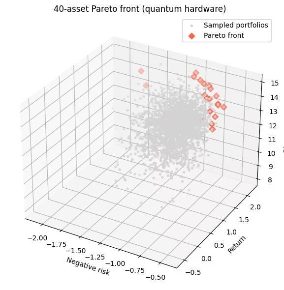
Feasible portfolios collected : 2359
Pareto-front portfolios       : 20
# --- Honest benchmark: QAOA and random vs the EXACT Pareto front ---
# 40 choose 6 = 3,838,380 feasible portfolios -- few enough to enumerate exactly, score
# every one on the TRUE objectives, and get the exact Pareto front. That front is an
# absolute ceiling, and its feasible nadir is a FIXED hypervolume reference point, so the
# numbers are comparable across runs instead of depending on what happened to be sampled.
import itertools

# Stream the combinations straight into an (n, K) index array, without first
# building millions of Python tuples.
combos = np.fromiter(
    itertools.chain.from_iterable(
        itertools.combinations(range(n_assets_40), K_40)
    ),
    dtype=np.int16,
).reshape(-1, K_40)
fis_exact = score_40(combos)
front_exact = filter_dominated(fis_exact, maximise=True)

# Fixed reference = worst value of each objective over ALL feasible portfolios (the nadir).
ref_fixed = fis_exact.min(axis=0)
# The hypervolume of a point set equals the hypervolume of its front.
hv_ceiling = hypervolume(front_exact, ref=ref_fixed, maximise=True)
hv_qaoa = hypervolume(fis_40, ref=ref_fixed, maximise=True)

def random_feasible_hv(n_draw, seed):
    """Hypervolume of n_draw uniformly-random feasible portfolios, same fixed reference."""
    rng = np.random.default_rng(seed)
    picks = set()
    while len(picks) < n_draw:
        picks.add(tuple(sorted(rng.choice(n_assets_40, K_40, replace=False))))
    P = np.array(list(picks))
    return hypervolume(score_40(P), ref=ref_fixed, maximise=True)

hv_rand = np.array(
    [random_feasible_hv(len(feasible_40), seed) for seed in range(20)]
)

print(f"Exact Pareto front            : {len(front_exact)} portfolios")
print(f"Hypervolume ceiling (optimum) : {hv_ceiling:.3f}")
print(
    f"QAOA (hardware)               : {100 * hv_qaoa / hv_ceiling:5.1f}% of optimum"
)
print(
    f"Random ({len(feasible_40)} draws, 20 seeds) : "
    f"{100 * hv_rand.mean() / hv_ceiling:5.1f}% +/- {100 * hv_rand.std() / hv_ceiling:.1f}% of optimum"
)
Exact Pareto front            : 61 portfolios
Hypervolume ceiling (optimum) : 64.211
QAOA (hardware)               :  85.5% of optimum
Random (2359 draws, 20 seeds) :  84.4% +/- 1.3% of optimum
Sa laking ito ng problema, halos kasing-husay ng uniform random sampling ang QAOA. Pareho silang nakakabawi ng malaking bahagi ng hypervolume ng exact na optimum, at walang malinaw na nangunguna. Inaasahan ang resultang ito para sa isang mababaw na QAOA layer na may lubhang pinutol na cost operator sa maingay na hardware; ang halaga ng halimbawang ito ay ang end-to-end na multi-objective workflow (mapping, angle training, constrained sampling, at Pareto post-processing), hindi ang quantum speed-up. Ang pagpapaliit ng agwat sa optimum ay mangangailangan ng mas malalalim na circuit (mas maraming QAOA layer), mas banayad na truncation, o hardware na mas mababa ang noise.
# The best trade-offs found by the sampler: no other sampled portfolio beats these
# on every objective. They approximate the exact front computed above; a
# decision-maker picks the trade-off they prefer.
bs_list = list(feasible_40)
# Boolean mask over fis_40; keep_weakly=True also keeps portfolios whose
# objective values tie with a front point (what the strict filter would drop).
mask = is_nondominated(fis_40, maximise=True, keep_weakly=True)
front_bs = [b for b, m in zip(bs_list, mask) if m]
front_f = fis_40[mask]
order = np.argsort(-front_f[:, 1])  # show a span sorted by return
print(
    f"{mask.sum()} non-dominated sampled portfolios. A representative span:\n"
)
print(
    f"{'tickers held':40s} {'risk':>7s} {'return':>7s} {'cross-sector':>12s}"
)
for idx in order[:: max(1, len(order) // 12)]:
    held = [tickers_40[i] for i, b in enumerate(front_bs[idx]) if b == "1"]
    print(
        f"{', '.join(held):40s} {-front_f[idx,0]:7.3f} {front_f[idx,1]:7.2f} {int(front_f[idx,2]):12d}"
    )

fig = plt.figure(figsize=(8, 6))
ax = fig.add_subplot(111, projection="3d")
ax.scatter(
    fis_40[:, 0],
    fis_40[:, 1],
    fis_40[:, 2],
    c="lightgray",
    s=8,
    label="Sampled portfolios",
)
ax.scatter(
    pareto_40[:, 0],
    pareto_40[:, 1],
    pareto_40[:, 2],
    c="tomato",
    marker="D",
    s=40,
    label="Pareto front",
)
ax.set_xlabel("Negative risk")
ax.set_ylabel("Return")
ax.set_zlabel("Diversification")
ax.set_title("40-asset Pareto front (quantum hardware)")
ax.legend()
plt.tight_layout()
plt.show()
20 non-dominated sampled portfolios. A representative span:

tickers held                                risk  return cross-sector
AAPL, NVDA, XOM, GS, BLK, CAT              1.715    2.22           13
NVDA, GS, MS, PFE, CAT, PLD                1.772    2.20           14
NVDA, MS, PFE, WMT, CAT, DUK               1.040    2.14           15
NVDA, CVX, GS, JNJ, KO, WMT                0.737    2.01           14
NVDA, COP, GS, JNJ, WMT, EQIX              1.014    1.98           15
NVDA, ABT, WMT, CAT, AEP, EQIX             0.913    1.92           15
NVDA, CVX, WMT, RTX, D, EQIX               0.835    1.82           15
NVDA, XOM, GS, JNJ, DUK, EQIX              0.763    1.80           15
AAPL, NVDA, JNJ, KO, RTX, SO               0.621    1.71           14
NVDA, CVX, BLK, JNJ, RTX, AEP              0.719    1.71           15
NVDA, JNJ, KO, COST, RTX, AEP              0.545    1.69           14
NVDA, CVX, ABT, WMT, HON, AEP              0.702    1.43           15
AAPL, GS, JNJ, PEP, AEP, EQIX              0.645    1.34           15
MSFT, XOM, BLK, JNJ, CAT, SO               0.617    1.34           15
MSFT, KO, WMT, RTX, SO, SPG                0.526    1.29           14
MSFT, XOM, BLK, JNJ, WMT, DUK              0.483    1.25           15
MSFT, CVX, JNJ, RTX, DUK, D                0.482    1.02           14
MSFT, XOM, JNJ, KO, HON, EQIX              0.479    0.93           15
MSFT, JNJ, PG, KO, RTX, DUK                0.423    0.86           14
MSFT, XOM, JNJ, PEP, DUK, AMT              0.476    0.57           15
Mga susunod na hakbang
Kung naging kawili-wili sa iyo ang tutorial na ito, isaalang-alang ang mga sumusunod:
-
Palitan ang na-download na market data (
market_data.csv) ng sarili mong mga return at covariance estimate mula sa totoong kasaysayan ng presyo. -
Dagdagan ang bilang ng mga QAOA layer, o magsanay sa 12–16 na asset at ilipat ang mga angle na iyon, para mailapit ang hardware front sa optimal.
-
Basahin ang Kotil et al., Quantum Approximate Multi-Objective Optimization (Nature Computational Science, 2025), ang max-cut na pag-aaral na iniaangkop ng tutorial na ito sa mga portfolio.
Mga sanggunian
-
Kotil et al., "Quantum Approximate Multi-Objective Optimization," Nature Computational Science (2025). arXiv:2503.22797
-
S. H. Sack at M. Serbyn, "Quantum annealing initialization of the quantum approximate optimization algorithm," Quantum 5, 491 (2021). arXiv:2101.05742