Shadow tomography ng Greenberger-Horne-Zeilinger state

Tantiya ng paggamit: Wala pang 10 segundo sa isang Heron r2 processor (PAALALA: Tantiya lamang ito. Maaaring mag-iba ang runtime mo.)

Mga learning outcome

• Kung paano bumubuo ang shadow tomography ng classical shadow ng isang quantum state at kung bakit exponential na mas kaunting measurement ang kailangan nito kaysa sa buong state tomography

• Kung paano mag-implement ng local Pauli shadow tomography gamit ang Qiskit para i-estimate ang single-qubit magnetization, two-point correlator, at two-qubit reduced density matrix

• Kung paano gamitin ang qiskit-paulice para sa low-overhead na error detection gamit ang spacetime code sa isang malakihang hardware experiment

Mga prerequisite

• Mga Measurement

• Quantum state tomography

• Error detection gamit ang spacetime code

Background

Ang buong quantum state tomography ng isang $N$-qubit na sistema ay nangangailangan ng exponential na dami ng measurement para i-estimate ang lahat ng $4^N -1$ na independent na parameter ng density matrix. Para sa sistemang may 50 qubit, halimbawa, nangangailangan ang prosesong ito ng humigit-kumulang $10^{30}$ shot, na higit sa isang bilyong beses ng bilang ng mga bituin sa observable universe. Ang shadow tomography [1] ay isang quantum information protocol na bumubuo ng “classical shadow” ng quantum state, kung saan maaaring i-estimate ang mga target na observable gamit ang bilang ng shot na logarithmic ang scaling sa bilang ng mga observable at independent sa laki ng sistemang $N$, kaya mahalaga ito sa maraming larangan ng quantum computing, kabilang ang energy estimation, entanglement entropy at correlation function calculation, kernel estimation sa quantum machine learning, at iba pa.

Ipinapakita ng tutorial na ito kung paano gamitin ang shadow tomography para i-estimate ang mga local observable, tulad ng single-qubit magnetization na $\langle Z_i \rangle$ para sa qubit na $i$, ang two-point correlation function na $\langle Z_i Z_j\rangle$, at ang two-qubit reduced density matrix (2-RDM), ng lubhang entangled na Greenberger-Horne-Zeilinger (GHZ) state. Una, ipinapakita ng tutorial ang maliit na shadow tomography workflow sa 10-qubit na GHZ state gamit ang statevector simulation. Pagkatapos, nagpapakita ito ng 100-qubit na demonstrasyon sa totoong quantum hardware.

Shadow tomography protocol

Ang shadow tomography protocol ay may mga sumusunod na hakbang:

1. Mag-apply ng random na unitary na $U$, na kinuha mula sa isang unitary ensemble, sa initial quantum state.
2. Sukatin ang resulta sa computational basis, para makakuha ng bitstring na $\ket{b}$.
3. Itabi ang classical snapshot, $\hat{\rho} = \mathcal{M}^{-1}(U^{\dagger}\ket{b}\bra{b}U)$, kung saan ang $\mathcal{M}^{-1}$ ay ang inverse ng measurement channel na $\mathcal{M}(\rho)=\mathbb{E}[U^{\dagger}\ket{b}\bra{b}U]$.
4. Ulitin ang proseso nang $T$ beses, kung saan ang koleksyon ng $T$ snapshot na $\{\hat{\rho}_t\}$ ay bumubuo ng classical shadow na $S(\rho, T)$.
5. I-estimate ang observable na $o$ ng operator na $O$ bilang $\frac{1}{T}\sum_{t=1}^{T}\text{Tr}(O\hat{\rho}_t)$.

Mga variant ng shadow tomography

Ang pagpili ng unitary ensemble, ibig sabihin ang basis, sa hakbang 1 ng protocol, ay nakakaapekto sa sample complexity, variance ng mga estimate, at pagkakumpleto ng impormasyon ng isang shadow tomography. Maraming ensemble group ang nasuri na sa literatura, na bawat isa ay may mga trade-off sa pagitan ng complexity at kahusayan ng observable estimation. Ibinubuod sa sumusunod na talahanayan ang mga katangian ng mga pinakakaraniwang ginagamit na variant, bagaman hindi kumpleto ang listahang ito.

Variant	Ensemble	Sample complexity	Circuit depth	Angkop na mga observable
local Pauli [1]	single-qubit Paulis $\{X, Y, Z\}$	$\mathcal{O}(3^k\text{log}M/\varepsilon^2)$	1	local/few-body
global Clifford [1]	$N$-qubit Clifford	$\mathcal{O}(\text{Tr}(O^2)\text{log}M/\varepsilon^2)$	$\mathcal{O}(N\text{log}N)$	low-rank, fidelity
fermionic Gaussian [2], [3]	matchgate circuits	$\mathcal{O}(\binom{\mu}{k}\frac{1}{\varepsilon^2})$	$\mathcal{O}(N^2)$	fermionic
shallow shadows [4], [5]	low-depth circuits	$\mathcal{O}(k2^k\text{log}M/\varepsilon^2)$	$\mathcal{O}(\text{log}N)$	non-local (hardware-friendly)

Ang mga terminong ginamit sa talahanayan ay tinutukoy bilang sumusunod:

• Ang "sample complexity" ay tumutukoy sa bilang ng mga measurement na kailangan para sa isang partikular na shadow tomography variant.

• Inilalarawan ng "circuit depth" kung gaano kamahal ipatupad ang mga measurement sa quantum hardware.

• Ang $N$ ay ang bilang ng mga qubit.

• Ang $k$ ay ang locality ng observable (halimbawa, ang $\langle Z_i \rangle$ ay may $k=1$ at ang $\langle Z_i Z_j\rangle$ ay may $k=2$).

• Ang $M$ ay ang bilang ng mga observable na sabay na ie-estimate.

• Ang $\varepsilon$ ay ang additive error tolerance.

• Ang $\mu$ ay ang bilang ng mga fermion.

Bagaman ang local Pauli ensemble ang pinaka-hardware-friendly, may kapalit itong $3^k$ na sample complexity penalty, kaya hindi ito angkop sa pag-estimate ng mga non-local na katangian. Mas pangkalahatan, ang local-shadow sample-complexity bound ay sumasabay sa $4^k$, na bumubuti sa $3^k$ sa espesyal na kaso ng mga tensor-product observable.

Sa kabilang banda, bagaman magagamit ang global Clifford ensemble para i-estimate ang mga non-local na observable, hindi paborable ang circuit depth nito. Nag-aalok ang mga fermionic Gaussian shadow ng gamit sa mga simulation ng many-body physics, chemistry, at materials, pero nangangailangan ng mga matchgate circuit, na maaaring magdala ng malaking overhead sa mga general purpose na gate-based na device.

Ang shallow shadows ay may circuit depth sa pagitan ng local Pauli at global Clifford, kaya isa itong lubhang promising na variant para sa praktikal na implementasyon, bagaman may ilang bukas pang tanong tungkol sa pinakamainam na circuit depth para sa isang partikular na observable.

Habang patuloy na lumalawak ang hangganan ng pananaliksik sa shadow tomography, kabilang sa pinakamahahalagang problemang tutugunan ang pinakamainam na pagpili ng measurement ensemble para sa target na hanay ng mga observable, pagpapabuti ng mga sample complexity bound, at pagpapalawak ng protocol sa mga time-evolved na observable. Gayunpaman, isa pa rin ang shadow tomography sa mga nangungunang workflow para kunin ang pinakamaraming classical na impormasyon mula sa isang quantum state gamit ang pinakakaunting measurement, kaya mainam ito sa pagkilala ng mga quantum state sa sukat kung saan imposible ang parehong buong tomography at classical simulation.

Ang local Pauli ensemble

Ginagamit ng tutorial na ito ang random Pauli basis, ibig sabihin ang mga single-qubit Clifford gate, para mangolekta ng mga shadow at mag-estimate ng mga katangian ng GHZ state. Tandaan na mahusay na pagpipilian ang mga Pauli measurement para sa pag-estimate ng mga local observable (tulad ng spin density, local correlation function, at position probability density), pero hindi para sa mga global (tulad ng total energy, momentum, at charge).

Dito, independiyenteng pumipili ng random na Pauli basis na $\{X, Y, Z\}$ bawat qubit at ina-apply ang katumbas na single-qubit rotation, na sinusundan ng measurement:

$$\begin{equation} U = U_0 \otimes U_1 \otimes \cdots \otimes U_{n-1}, U_q \in \{I, H, S^{\dagger}H\} \end{equation} \tag{1}$$

Para sa ensemble na ito, ang inverse ng measurement channel ay:

$$\begin{equation} \hat{\rho}_q=3U_q^{\dagger}\ket{b_q}\bra{b_q}U_q - I \end{equation} \tag{2}$$

Ang factor na $3$ ay nagmumula sa pag-average sa tatlong Pauli basis, na gumagawa ng depolarizing channel na may parameter na $\frac{1}{3}$. Pagkatapos, nagfa-factorize ang buong estimator bilang produkto ng mga single-qubit estimator. Gaya ng ipinapakita sa talahanayan, para sa $M$ na observable, na bawat isa ay may locality na $k$, ang bilang ng mga Pauli shadow na kailangan para i-estimate ang lahat ng observable hanggang additive error na $\varepsilon$ nang may mataas na probabilidad ay $\mathcal{O}(\frac{3^k\text{log}(M)}{\varepsilon^2})$. Hindi nakakaapekto ang laki ng sistema sa gastos ng measurement basta nananatiling local ang mga observable, kaya maaaring sabay na i-estimate ang exponential na dami ng observable sa logarithmic na gastos lamang.

Median of means

Binabawasan ng payak na mean sa $T$ snapshot ang variance ng single-shot na estimate ng isang observable bilang $\frac{1}{T}$, pero sensitibo ito sa mga outlier. Magagamit ang median of means para lunasan ito. Kasama sa proseso ang sumusunod:

• Paghahati ng $T$ snapshot sa $K$ grupong pantay ang laki
• Pagkalkula ng mean sa loob ng bawat grupo
• Pagbabalik ng median sa mga mean ng mga grupo

Nagsasagawa ang tutorial na ito ng local Pauli shadow tomography para i-estimate ang mga katangian ng GHZ state, una gamit ang 10-qubit na simulated na halimbawa at pagkatapos ay nagpapakita ng 100-qubit na hardware experiment.

Mga kinakailangan

Bago simulan ang tutorial na ito, tiyaking naka-install ang mga sumusunod:

• Qiskit SDK v2.0 o mas bago, na may suporta sa visualization

• IBM Quantum Compute v0.28 o mas bago (pip install qiskit-ibm-runtime)

• Qiskit Paulice (pip install qiskit-paulice)

Setup

# Added by doQumentation — installs the packages this notebook needs if they are missing
import importlib.util

_needed = {"matplotlib": "matplotlib", "numpy": "numpy", "qiskit": "qiskit", "qiskit_ibm_runtime": "qiskit-ibm-runtime", "qiskit_paulice": "qiskit-paulice"}
_missing = [pip for module, pip in _needed.items()
            if importlib.util.find_spec(module) is None]
# One at a time, so a package that fails to install does not block the others
for _pip in _missing:
    %pip install -q {_pip}
if not _missing:
    print("\u2713 All required packages are installed")

import numpy as np
import matplotlib.pyplot as plt
from collections import deque, defaultdict
from qiskit import QuantumCircuit, ClassicalRegister
from qiskit.quantum_info import (
    Statevector,
    partial_trace,
    Operator,
    Pauli,
    SparsePauliOp,
)
from qiskit.transpiler import generate_preset_pass_manager
from qiskit_ibm_runtime import QiskitRuntimeService
from qiskit_ibm_runtime import SamplerV2 as Sampler
from qiskit_paulice.layout import get_low_overhead_ancillas

seed = 42  # for reproducibility
rng = np.random.default_rng(seed)

Ginagamit ang mga sumusunod na helper function sa malakihang hardware example mamaya sa tutorial:

• bad_cz, bad_readout, bad_coherence — Nagqu-query ng backend calibration data para tukuyin ang mga gate, qubit, at edge na lumalampas sa mga error o coherence threshold, para maibukod ang mga ito sa circuit layout.

• parallel_ghz — Bumubuo ng GHZ circuit na may ibinigay na laki gamit ang breadth-first search sa coupling map, na nagpapakalat ng mga CNOT layer nang parallel para mabawasan ang circuit depth.

• weighted_coverage, active_wires, z_trace_backward — Kinukwenta kung gaano karami sa error surface ng GHZ circuit ang protektado ng isang hanay ng mga spacetime parity check, gamit ang backward-propagation technique mula sa [6].

• add_measurements — Nagdaragdag ng mga measurement ng GHZ-qubit at check-qubit sa magkahiwalay na classical register para maaari silang i-postselect nang magkahiwalay.

• build_shadow_circuits — Gumagawa ng isang circuit bawat random Pauli basis sa pamamagitan ng pagdaragdag ng angkop na mga single-qubit rotation bago ang measurement.

• parse_hw_results_w_checks — Ina-unpack ang output ng Sampler sa mga triple na (ghz_bits, check_bits, bases), isa bawat shot.

• adapt_to_flat_bits, estimate_zz_nn_hw — Ima-map pabalik ang mga bit ng GHZ-register sa buong index space ng device at kinukwenta ang median-of-means na estimate ng $\langle Z_i Z_{i+1}\rangle$.

def bad_cz(target, threshold: float = 0.01) -> list:
    "Return edges whose CZ error exceeds threshold."
    edges = []
    for edge in backend.target.build_coupling_map().get_edges():
        if (edge[1], edge[0]) not in edges:
            edges.append(edge)
    cz_errors = {edge: target["cz"][edge].error for edge in edges}
    worst = sorted(cz_errors.items(), key=lambda x: x[1], reverse=True)
    return [list(edge) for edge, error in worst if error > threshold]

def bad_readout(target, threshold: float = 0.01) -> list:
    "Return nodes whose measurement error exceeds threshold."
    meas_errors = {
        node: target["measure"][(node,)].error
        for node in range(backend.num_qubits)
    }
    worst = sorted(meas_errors.items(), key=lambda x: x[1], reverse=True)
    return [node for node, error in worst if error > threshold]

def bad_coherence(target, threshold: float = 60) -> list:
    "Return nodes whose T2 value is below threshold."
    t2s = {
        node: (target.qubit_properties[node].t2 or 0) * 1e6
        for node in range(backend.num_qubits)
    }
    return [
        node
        for node, val in sorted(t2s.items(), key=lambda x: x[1])
        if val < threshold
    ]

def parallel_ghz(
    root: int, num_qubits: int, backend, bad_edges: list, skip: list
) -> tuple:
    "Build a GHZ circuit of size num_qubits using BFS from root, one neighbor per layer."
    edges = [
        e
        for e in [list(e) for e in backend.coupling_map.get_edges()]
        if e not in bad_edges
        and [e[1], e[0]] not in bad_edges
        and e[0] not in skip
        and e[1] not in skip
    ]
    adj = defaultdict(list)
    for u, v in edges:
        adj[u].append(v)
        adj[v].append(u)

    qc = QuantumCircuit(backend.num_qubits)
    visited = [root]
    queue = deque([root])
    explored = defaultdict(set)
    layers = []
    qc.h(root)

    while queue and len(visited) < num_qubits:
        layer = []
        for node in list(queue):
            queue.popleft()
            unvisited = [
                nb
                for nb in adj[node]
                if nb not in visited and nb not in explored[node]
            ]
            if unvisited:
                nb = unvisited[0]
                visited.append(nb)
                queue.append(node)
                queue.append(nb)
                explored[node].add(nb)
                layer.append((node, nb))
                if len(visited) == num_qubits:
                    break
        if layer:
            layers.append(layer)
        else:
            break

    for layer in layers:
        for q1, q2 in layer:
            qc.cx(q1, q2)
        qc.barrier()

    return qc, visited, layers

def weighted_coverage(
    layers: list, parities: list, w_idle: float = 0.2, w_gate: float = 0.8
) -> float:
    "Compute weighted fraction of wires covered by at least one parity check."
    wires = active_wires(layers)
    covered_by_any = {n_layer: set() for n_layer in range(len(layers))}
    for parity in parities:
        for n_layer, qs in z_trace_backward(layers, parity).items():
            covered_by_any[n_layer] |= qs
    covered_weight = total_weight = 0
    for n_layer in range(len(layers)):
        idle = wires[n_layer]["idle"]
        gate = wires[n_layer]["gate"]
        total_weight += w_idle * len(idle) + w_gate * len(gate)
        covered_weight += w_idle * len(
            covered_by_any[n_layer] & idle
        ) + w_gate * len(covered_by_any[n_layer] & gate)
    return covered_weight / total_weight if total_weight > 0 else 0

def active_wires(layers: list) -> dict:
    """
    Returns per-layer dict with two sets:
    - 'idle': activated wires that are idle in this layer
    - 'gate': activated wires that are control/target of a CNOT at this layer
    """
    first_activation = {}
    for n_layer, layer in enumerate(layers):
        for c, t in layer:
            first_activation.setdefault(c, n_layer)
            first_activation.setdefault(t, n_layer)
    result = {}
    for n_layer in range(len(layers)):
        active = {
            q
            for q, n_layer0 in first_activation.items()
            if n_layer >= n_layer0
        }
        gate = {q for c, t in layers[n_layer] for q in (c, t)}
        result[n_layer] = {"idle": active - gate, "gate": gate}
    return result

def z_trace_backward(layers: list, initial_Zs: list) -> dict:
    """
    Backward propagate Zs with parity cancellation.
    Returns {layer: set of qubits with odd parity Z at that layer}.
    """
    wires = active_wires(layers)
    support = set(initial_Zs)
    trace = {}
    for n_layer in range(len(layers) - 1, -1, -1):
        active = wires[n_layer]["idle"] | wires[n_layer]["gate"]
        trace[n_layer] = support & active
        new_support = set()
        for q in support:
            hit = False
            for c, t in layers[n_layer]:
                if q == t:
                    new_support ^= {t, c}
                    hit = True
                    break
                elif q == c:
                    new_support ^= {c}
                    hit = True
                    break
            if not hit:
                new_support ^= {q}
        support = new_support
    return trace

def add_measurements(
    qc: QuantumCircuit, ghz_qubits: list, checks: list
) -> QuantumCircuit:
    "Add GHZ and check qubit measurements into separate classical registers."
    c1 = ClassicalRegister(len(ghz_qubits), "c1")
    qc.add_register(c1)
    for q, c in zip(ghz_qubits, c1):
        qc.measure(q, c)
    c2 = ClassicalRegister(len(checks), "c2")
    qc.add_register(c2)
    for q, c in zip(checks, c2):
        qc.measure(q, c)
    return qc

def build_shadow_circuits(
    base_circuit: QuantumCircuit,
    n_measure: int,
    ghz_qubits: list,
    checks: list,
) -> tuple:
    "Build n_measure circuits by appending random Pauli basis rotations to each GHZ qubit."
    n = base_circuit.num_qubits
    all_bases = rng.integers(0, 3, size=(n_measure, n))
    circuits = []
    for m in range(n_measure):
        qc = base_circuit.copy()
        qc.barrier()
        for q in ghz_qubits:
            b = all_bases[m, q]
            if b == 1:
                qc.h(q)
            elif b == 2:
                qc.sdg(q)
                qc.h(q)
        add_measurements(qc, ghz_qubits, checks)
        circuits.append(qc)
    return circuits, all_bases

def parse_hw_results_w_checks(
    result, bases: np.ndarray, ghz_qubits: list, checks: list
) -> list:
    "Parse hardware bitstrings into (ghz_bits, check_bits, bases) triples."
    snapshots = []
    n_ghz = len(ghz_qubits)
    n_checks = len(checks)
    for t, pub_result in enumerate(result):
        ghz_strings = (
            pub_result.data.c1.get_bitstrings()
        )  # one entry per shot
        chk_strings = pub_result.data.c2.get_bitstrings()
        for ghz_bitstring, check_bitstring in zip(ghz_strings, chk_strings):
            ghz_bits = [
                int(ghz_bitstring[n_ghz - 1 - i]) for i in range(n_ghz)
            ]
            check_bits = [
                int(check_bitstring[n_checks - 1 - i])
                for i in range(n_checks)
            ]
            snapshots.append((ghz_bits, check_bits, bases[t]))
    return snapshots

def adapt_to_flat_bits(
    ghz_bits: list, ghz_qubits: list, n_total: int
) -> list:
    "Map GHZ-register bits back to a full n_total-length bit vector."
    bits = [0] * n_total
    for i, q in enumerate(ghz_qubits):
        bits[q] = ghz_bits[i]
    return bits

def estimate_zz_nn_hw(
    snapshots: list, ghz_qubits: list, n_total: int, n_groups: int
) -> np.ndarray:
    "Estimate <ZiZi+1> for each neighboring GHZ qubit pair from flat-bit snapshots."
    pairs = list(zip(ghz_qubits[:-1], ghz_qubits[1:]))
    all_est = np.column_stack(
        [
            snapshot_estimate(
                ["Z" if q in pair else "I" for q in range(n_total)], snapshots
            )
            for pair in pairs
        ]
    )
    return mom(all_est, n_groups).real

Maliit na simulator example

Una, maghanda ng 10-qubit na GHZ state gamit ang statevector simulation at i-estimate ang mga katangian nito gamit ang mga local Pauli shadow. Ang GHZ state ay isang maximally entangled na quantum state na may tatlo o higit pang qubit na nagsisilbing benchmark para sa multipartite entanglement. Karaniwan itong building block para sa mga quantum communication at cryptography protocol. Bukod dito, ang GHZ circuit ay may ganap na kilalang analytical na mga katangian, kaya mainam ito para sa verification sa tutorial na ito.

Hakbang 1: I-map ang mga classical input sa isang quantum problem

Maghanda ng ideal na 10-qubit na GHZ state.

def ghz_statevector(num_qubits):
    qc = QuantumCircuit(num_qubits)
    qc.h(0)
    for q in range(num_qubits - 1):
        qc.cx(q, q + 1)
    return Statevector(qc)

num_qubits = 10  # number of qubits
psi = ghz_statevector(num_qubits)
psi.seed(seed)
print(
    f"{num_qubits}-qubit GHZ state ready (norm = {np.linalg.norm(psi):.6f})"
)

10-qubit GHZ state ready (norm = 1.000000)

Hakbang 2: I-optimize para sa pagpapatakbo sa quantum hardware

Susunod, mag-define ng function na nangongolekta ng mga shadow snapshot sa pamamagitan ng pag-rotate ng GHZ state sa mga random na Pauli basis. Ginagaya nito ang ginagawa ng Sampler primitive sa hardware sa malakihang halimbawa.

def basis_circuit(b):
    """0 -> Z basis (I), 1 -> X basis (H), 2 -> Y basis (Sdg;H)."""
    qc = QuantumCircuit(1)
    if b == 1:
        qc.h(0)
    elif b == 2:
        qc.sdg(0)
        qc.h(0)
    # b == 0: Z basis, no rotation
    return qc

_basis = {
    b: basis_circuit(b) for b in (0, 1, 2)
}  # built once, shared with the estimator's _U

def collect_shadow_snapshots(psi, n_snapshots, num_qubits):
    snapshots = []
    for _ in range(n_snapshots):
        bases = rng.integers(0, 3, size=num_qubits)
        rot = QuantumCircuit(num_qubits)
        for q, b in enumerate(bases):
            rot.compose(_basis[b], qubits=[q], inplace=True)
        evolved = psi.evolve(rot)
        evolved.seed(int(rng.integers(0, 2**31)))
        bitstr = next(
            iter(evolved.sample_counts(shots=1))
        )  # Born rule internal
        bits = [int(x) for x in bitstr[::-1]]  # little-endian -> qubit
        snapshots.append((bits, bases))
    return snapshots

Hakbang 3: Patakbuhin gamit ang mga Qiskit primitive

Para sa simulation na ito, gamitin nang direkta ang statevector.

n_snapshots = 5000  # number of shadow snapshots
n_groups = 20  # groups/batches for median-of-means

snapshots = collect_shadow_snapshots(psi, n_snapshots, num_qubits)
print(f"Collected {n_snapshots} snapshots.")

Collected 5000 snapshots.

Hakbang 4: I-post-process at ibalik ang resulta sa nais na classical na format

Tukuyin ang shadow estimator at ang median-of-means (MOM) estimator para sa mga random na measurement basis na ginamit sa pagkolekta ng mga shadow snapshot. Gamitin ang mga function na ito para tantiyahin ang mga katangian ng GHZ state, kasama ang single-qubit magnetization, two-qubit correlator, at two-qubit RDM, mula sa mga nakolektang measurement. Pagkatapos, ihambing ang mga tantiya sa eksaktong mga halaga.

_U = {
    b: Operator(basis_circuit(b)) for b in (0, 1, 2)
}  # rotation Uᵢ per basis
_P = {p: Operator(Pauli(p)) for p in "IXYZ"}  # single-qubit Paulis

def shadow_estimator(P, b, bit):  # P is a label char, e.g. "X"
    UPU = _U[b] @ _P[P] @ _U[b].adjoint()  # Uᵢ P Uᵢ†
    return (3 * UPU.data[bit, bit] - np.trace(_P[P].data)).real

def mom(estimates: np.ndarray, n_groups: int) -> np.ndarray:
    "Median-of-means outlier suppression."
    T = len(estimates)
    spg = T // n_groups  # shots per group
    trimmed = estimates[
        : spg * n_groups
    ]  # drop any leftover shots that don't cleanly fit into a group
    groups = trimmed.reshape(n_groups, spg, *estimates.shape[1:])
    means = groups.mean(axis=1)  # take the mean of each group
    return np.median(means.real, axis=0) + 1j * np.median(
        means.imag, axis=0
    )  # take the median of means for real and imaginary parts separately

def snapshot_estimate(
    pauli_string, snapshots
):  # full-width label, len == num_qubits
    out = np.empty(len(snapshots), dtype=complex)
    for t, (bits, bases) in enumerate(snapshots):
        e = 1.0 + 0j
        for q, P in enumerate(pauli_string):
            e *= shadow_estimator(P, bases[q], bits[q])
        out[t] = e
    return out

Z_est = np.column_stack(
    [
        snapshot_estimate(
            ["Z" if q == i else "I" for q in range(num_qubits)], snapshots
        )
        for i in range(num_qubits)
    ]
)
Z_vals = mom(Z_est, n_groups).real

ZZ_est = np.column_stack(
    [
        snapshot_estimate(
            ["Z" if q in (i, i + 1) else "I" for q in range(num_qubits)],
            snapshots,
        )
        for i in range(num_qubits - 1)
    ]
)
ZZ_nn = mom(ZZ_est, n_groups).real

ZZ_full = np.zeros((n_snapshots, num_qubits, num_qubits), dtype=complex)
for i in range(num_qubits):
    ZZ_full[:, i, i] = 1.0  # diagonal is always 1
    for j in range(i + 1, num_qubits):
        col = snapshot_estimate(
            ["Z" if q in (i, j) else "I" for q in range(num_qubits)],
            snapshots,
        )
        ZZ_full[:, i, j] = col
        ZZ_full[:, j, i] = col  # symmetric
ZZ_mat = mom(ZZ_full, n_groups).real

# 2-qubit reduced density matrix (RDM) for pair (qi, qj)
# the elementwise complex median (real/imag split) for the RDM coefficients generalizes the scalar median in Ref.[1]
qi, qj = 0, num_qubits - 1
terms = []
for a in "IXYZ":
    for b in "IXYZ":
        label = "".join({qi: a, qj: b}.get(q, "I") for q in range(num_qubits))
        c = mom(snapshot_estimate(label, snapshots).reshape(-1, 1), n_groups)[
            0
        ]
        terms.append((b + a, c / 4))
rho_shadow = SparsePauliOp.from_list(terms).to_matrix()

traced_out = [q for q in range(num_qubits) if q not in (qi, qj)]
rho_exact = partial_trace(
    psi, traced_out
).data  # diag(0.5, 0, 0, 0.5) for GHZ

print(f"{'Observable':<22} {'Estimated':>12} {'Ideal':>8} {'Max error':>12}")
print("-" * 57)
print(
    f"{'<Zi> (all qubits)':<22} {'-':>12} {'0':>8} {np.max(np.abs(Z_vals)):>12.4f}"
)
print(
    f"{'<ZiZi+1> mean':<22} {np.mean(ZZ_nn):>12.4f} {'1':>8} {np.max(np.abs(ZZ_nn - 1)):>12.4f}"
)
print(
    f"{'2-RDM Frobenius err':<22} {'-':>12} {'0':>8} {np.linalg.norm(rho_shadow - rho_exact):>12.4f}"
)

Observable                Estimated    Ideal    Max error
---------------------------------------------------------
<Zi> (all qubits)                 -        0       0.0540
<ZiZi+1> mean                1.0040        1       0.1520
2-RDM Frobenius err               -        0       0.1080

I-visualize ang mga resulta

Ipinapakita ng unang plot ang tinantiyang mga halaga ng single-qubit magnetization para sa iba't ibang qubit. Ipinapakita ng pangalawang plot ang distribusyon ng tinantiyang mga halaga ng two-point correlator para sa lahat ng pares ng qubit. Ipinapakita ng huling plot ang magnitude ng mga entry ng two-qubit reduced density matrix. Medyo malaking koleksyon ng mga snapshot ang ginamit para sa laki ng sistema, kaya malapit sa eksakto ang mga resulta.

fig, axes = plt.subplots(
    1, 3, figsize=(14, 4), gridspec_kw={"width_ratios": [1, 1, 1]}
)

z_exact = psi.expectation_value(
    SparsePauliOp.from_sparse_list([("Z", [0], 1.0)], num_qubits)
).real  # 0.0
zz_exact = psi.expectation_value(
    SparsePauliOp.from_sparse_list([("ZZ", [0, 1], 1.0)], num_qubits)
).real  # 1.0

# <Zi>
axes[0].bar(range(num_qubits), Z_vals, color="#4a90d9", alpha=0.85)
axes[0].axhline(0, color="black", lw=0.8)
axes[0].set_ylim(-0.5, 0.5)
axes[0].set_title(r"$\langle Z_i \rangle$ (ideal = %0.2f)" % z_exact)
axes[0].set_xlabel("Qubit index")
axes[0].grid(axis="y", alpha=0.3)

# <ZiZj>
im = axes[1].imshow(ZZ_mat, vmin=-1, vmax=1, cmap="magma")
plt.colorbar(im, ax=axes[1])
axes[1].set_title(r"$\langle Z_i Z_j \rangle$ (ideal = %0.2f)" % zz_exact)
axes[1].set_xlabel("Qubit j")
axes[1].set_ylabel("Qubit i")

# 2-RDM magnitude
im2 = axes[2].imshow(np.abs(rho_shadow), vmin=0, vmax=0.5, cmap="Blues")
plt.colorbar(im2, ax=axes[2])
axes[2].set_title(r"$|\rho_2|$ for qubits (0, N-1)")
axes[2].set_xticks(range(4))
axes[2].set_yticks(range(4))
axes[2].set_xticklabels(["00", "01", "10", "11"])
axes[2].set_yticklabels(["00", "01", "10", "11"])

[Text(0, 0, '00'), Text(0, 1, '01'), Text(0, 2, '10'), Text(0, 3, '11')]

Suriin ang shot scaling

Sa tutorial na ito, 5,000 snapshot ang ginagamit para tantiyahin ang mga observable. Sinusuri ang shot scaling ng shadow tomography sa pamamagitan ng pag-plot ng mean error ng isa sa mga tinantiyang function laban sa iba't ibang shot budget. Ang error sa two-qubit correlator ay bumababa bilang $1/\sqrt{T}$, gaya ng inaasahan sa karaniwang statistical convergence ng isang mean estimator. Ang kahalagahan ng shadow tomography ay ang constant prefactor sa harap ng $1/\sqrt{T}$ ay hindi lumalaki kasabay ng bilang ng qubit para sa mga local observable, tulad ng mga sinuri sa tutorial na ito.

shot_counts = [100, 250, 500, 1000, 2000, 5000, 10000]
errors = []

for N_test in shot_counts:
    snaps = collect_shadow_snapshots(psi, N_test, num_qubits)
    zz_vals = []
    for i in range(num_qubits - 1):
        ests = []
        for bits, bases in snaps:
            e = 1.0 + 0j
            for q in range(num_qubits):
                op = "Z" if q in (i, i + 1) else "I"
                e *= shadow_estimator(op, bases[q], bits[q])
            ests.append(e.real)
        zz_vals.append(np.mean(ests))
    errors.append(float(np.mean(np.abs(np.array(zz_vals) - 1.0))))
    print(f"T={N_test:5d} error = {errors[-1]:.4f}")

fig, ax = plt.subplots(figsize=(6, 4))
T_arr = np.array(shot_counts, dtype=float)
ax.loglog(T_arr, errors, "o-", color="#4a90d9", lw=2, label="Shadow estimate")
ax.loglog(
    T_arr,
    errors[0] * np.sqrt(shot_counts[0] / T_arr),
    "k--",
    alpha=0.5,
    label=r"$1/\sqrt{T}$ reference",
)
ax.set_xlabel("Shots T")
ax.set_ylabel(r"Mean $|\langle Z_i Z_{i+1} \rangle - 1|$")
ax.set_title(f"Convergence for {num_qubits}-qubit GHZ")
ax.legend()
plt.tight_layout()
plt.show()

T=  100 error = 0.1856
T=  250 error = 0.1613
T=  500 error = 0.1027
T= 1000 error = 0.0827
T= 2000 error = 0.0513
T= 5000 error = 0.0311
T=10000 error = 0.0162

Halimbawa sa malaking-sukat na hardware

Kinukumpirma ng naunang simulation na naibabalik ng local Pauli shadow tomography ang tamang mga observable sa isang noiseless na statevector. Ang pagpapatakbo ng parehong protocol gamit ang 100 qubit sa totoong hardware ay nagdudulot ng dalawang hamon na wala sa simulation: nag-iipon ang mga error ng gate at readout sa buong malalim na GHZ circuit, at ang paghahanap ng pinakamainam na layout ng qubit ay nangangailangan ng paghahanap sa coupling graph ng device sa halip na pumili ng layout nang mano-mano.

Para tugunan ang unang hamon, gumamit ng low-overhead error detection gamit ang mga spacetime code [6]. Isang maliit na bilang ng mga ancilla qubit na katabi ng GHZ tree ang ginagamit bilang mga parity check. Ang bawat ancilla ay ine-entangle sa dalawa sa mga kapitbahay nitong GHZ bago ang measurement, kaya ang isang bit-flip error sa alinmang kapitbahay ay babaligtarin ang resulta ng ancilla mula 0 patungong 1. Itinatapon ang mga snapshot kung saan nagbabasa ng 1 ang anumang check ancilla, na nag-iiwan ng mas malinis na subset para tantiyahin ang $\langle Z_i Z_{i+1}\rangle$.

Ang pangalawang hamon ay tinutugunan sa pamamagitan ng paghahanap sa mga kandidatong layout ng GHZ tree at pagpili sa isa na nagpapalaki ng parity-check coverage, ibig sabihin, ang bahagi ng mga wire ng circuit na binabantayan ng kahit isang check, sa loob ng katanggap-tanggap na pagtaas ng circuit depth.

Mga Hakbang 1-4 (isinasagawa sa iisang code block)

Ang parehong four-step na workflow ay inilalapat na ngayon sa isang 100-qubit na GHZ state sa totoong quantum hardware, na nagdaragdag ng dalawang feature na partikular sa hardware na hindi lumilitaw sa simulation:

• Hakbang 1 ay nagpapakilala sa noise ng backend (mga error ng gate, mga error ng readout, at mga oras ng T2) para hindi isama sa layout ng circuit ang mga hindi maaasahang qubit at edge.

• Hakbang 2 ay naghahanap sa mga posibleng layout ng GHZ tree para makahanap ng isa na nagpapalaki ng parity-check coverage sa loob ng katanggap-tanggap na circuit depth — pinapalitan ang simpleng chain na ginamit sa simulation.

• Hakbang 3 ay bumubuo ng mga shadow circuit (isa para sa bawat random na Pauli basis), nagta-transpile sa mga ito sa mga hardware-native na gate, at nagsusumite sa mga ito sa Sampler primitive na may shots=8 (bawat circuit ay gumagawa ng walong independiyenteng bitstring).

• Hakbang 4 ay nagpo-postselect ng mga snapshot kung saan lahat ng check qubit ay nagbabasa ng 0 (walang natukoy na error), pagkatapos ay tinatantiya ang $\langle Z_i Z_{i+1}\rangle$ na mayroon at walang postselection na iyon para ipakita ang pagbuti mula sa error detection.

# ── Step 1: Map classical inputs to a quantum problem ─────────────────────────
service = QiskitRuntimeService()
backend = service.least_busy(
    operational=True, simulator=False, min_num_qubits=133
)
coupling_map = backend.target.build_coupling_map()
n_total = backend.num_qubits

thresh_cz, thresh_meas, thresh_t2 = 0.025, 0.15, 10
bad_edges = bad_cz(backend.target, threshold=thresh_cz)
bad_nodes_readout = bad_readout(backend.target, threshold=thresh_meas)
dead_qubits = bad_readout(backend.target, threshold=0.4)
bad_nodes = list(
    set(bad_nodes_readout)
    | set(bad_coherence(backend.target, threshold=thresh_t2))
)

# ── Step 2: Optimize for quantum hardware execution ───────────────────────────
# Search over starting qubits and random node-skip sets to find the GHZ layout
# with the best parity-check coverage within an acceptable circuit depth.
ghz_size = 100
max_skips, shuffles, max_depth_increase = 10, 200, 10
w_idle, w_gate = 0.2, 0.8

# Find the root that yields the shallowest GHZ — exclude bad_nodes from the start
best_root = None
base_depth = float("inf")
for root in range(backend.num_qubits):
    if root in bad_nodes:
        continue
    qc, ghz_qubits, _ = parallel_ghz(
        root, ghz_size, backend, bad_edges, bad_nodes
    )
    if len(ghz_qubits) != ghz_size:
        continue
    depth = qc.depth(lambda x: x.operation.num_qubits == 2)
    if depth < base_depth:
        best_root, base_depth = root, depth
if best_root is None:
    raise Exception(
        "No qualifying GHZ root layout found. Relax error thresholds."
    )

qc, ghz_qubits, layers = parallel_ghz(
    best_root, ghz_size, backend, bad_edges, bad_nodes
)

degree_two_nodes = [
    i
    for i in ghz_qubits
    if all(n in ghz_qubits for n in coupling_map.neighbors(i))
    and len(coupling_map.neighbors(i)) >= 2
]

best_covered_fraction = -1
best_qc = best_checks = best_parities = best_layers = best_ghz_qubits = None

for num_skips in range(max_skips):
    for _ in range(shuffles):
        skip_trial = list(
            rng.choice(degree_two_nodes, num_skips, replace=False)
        )
        qc, ghz_qubits, layers = parallel_ghz(
            best_root, ghz_size, backend, bad_edges, skip_trial + bad_nodes
        )
        if len(ghz_qubits) != ghz_size:
            continue
        depth = qc.depth(lambda x: x.operation.num_qubits == 2)
        checks, parities = [], []
        for ancilla, neighbors in get_low_overhead_ancillas(
            coupling_map, ghz_qubits
        ).items():
            if ancilla in dead_qubits:
                continue
            good_neighbors = [
                n
                for n in neighbors
                if [ancilla, n] not in bad_edges
                and [n, ancilla] not in bad_edges
            ]
            if len(good_neighbors) < 2:
                continue
            checks.append(ancilla)
            parities.append((good_neighbors[0], good_neighbors[1]))
            qc.cx(good_neighbors[0], ancilla)
            qc.cx(good_neighbors[1], ancilla)
        covered_fraction = weighted_coverage(
            layers=layers, parities=parities, w_idle=w_idle, w_gate=w_gate
        )
        if (
            covered_fraction > best_covered_fraction
            and depth <= base_depth + max_depth_increase
        ):
            best_covered_fraction = covered_fraction
            (
                best_qc,
                best_ghz_qubits,
                best_checks,
                best_parities,
                best_layers,
            ) = qc, ghz_qubits, checks, parities, layers

qc, ghz_qubits, checks, parities, layers = (
    best_qc,
    best_ghz_qubits,
    best_checks,
    best_parities,
    best_layers,
)
if len(ghz_qubits) != ghz_size:
    raise Exception("No GHZ found. Relax error thresholds.")

print(f"GHZ qubits: {ghz_qubits} ({len(ghz_qubits)})")
print(f"Check qubits: {checks} ({len(checks)})")
print(
    "Covered fraction (no idle): ",
    weighted_coverage(
        layers=layers, parities=parities, w_idle=0.0, w_gate=1.0
    ),
)

# ── Step 3: Execute using Qiskit primitives ───────────────────────────────────
# Build one shadow circuit per random Pauli basis, each repeated for shots_per_basis
# independent bitstrings. Transpile to hardware-native gates, then submit using the
# Sampler primitive. Each circuit yields shots_per_basis snapshots in that basis.
n_hw = 1000
shots_per_basis = 8  # multiple shots per basis circuit
shadow_circs, hw_bases = build_shadow_circuits(qc, n_hw, ghz_qubits, checks)
sampler = Sampler(backend)
sampler.options.environment.job_tags = ["TUT_STGHZS"]
pm = generate_preset_pass_manager(optimization_level=1, backend=backend)
isa_circuit = pm.run(shadow_circs)
job = sampler.run(isa_circuit, shots=shots_per_basis)
result = job.result()

# ── Step 4: Post-process and return result in desired classical format ─────────
# Filter snapshots whose check qubits all read 0 (no detected error), then
# estimate <ZiZi+1> with and without the error-detection postselection.
snapshots_hw = parse_hw_results_w_checks(result, hw_bases, ghz_qubits, checks)
snapshots_kept = [
    (ghz_bits, check_bits, bases)
    for (ghz_bits, check_bits, bases) in snapshots_hw
    if all(b == 0 for b in check_bits)
]
snapshots_kept_adapted = [
    (adapt_to_flat_bits(ghz_bits, ghz_qubits, n_total), bases)
    for (ghz_bits, check_bits, bases) in snapshots_kept
]
snapshots_hw_adapted = [
    (adapt_to_flat_bits(ghz_bits, ghz_qubits, n_total), bases)
    for (ghz_bits, check_bits, bases) in snapshots_hw
]

print("Shadow snapshots collected:", len(snapshots_hw))
print("Shadow snapshots kept post error-detection:", len(snapshots_kept))

n_groups = min(5, len(snapshots_kept))  # groups for median-of-means
ZZ_hw = estimate_zz_nn_hw(snapshots_hw_adapted, ghz_qubits, n_total, n_groups)
ZZ_kept = estimate_zz_nn_hw(
    snapshots_kept_adapted, ghz_qubits, n_total, n_groups
)

# Plot <ZiZi+1> before and after error detection
fig, axes = plt.subplots(1, 2, figsize=(13, 4))

axes[0].plot(ZZ_hw, "o-", color="#e05c5c", markersize=4)
axes[0].axhline(1.0, color="gray", ls="--", alpha=0.7, label="Ideal")
axes[0].set_ylim(-0.6, 3.0)
axes[0].set_title(r"$\langle Z_i Z_{i+1} \rangle$ (without error detection)")
axes[0].set_xlabel("GHZ qubit pair")
axes[0].legend()
axes[0].grid(alpha=0.3)

axes[1].plot(ZZ_kept, "o-", color="#e05c5c", markersize=4)
axes[1].axhline(1.0, color="gray", ls="--", alpha=0.7, label="Ideal")
axes[1].set_ylim(-0.6, 3.0)
axes[1].set_title(r"$\langle Z_i Z_{i+1} \rangle$ (with error detection)")
axes[1].set_xlabel("GHZ qubit pair")
axes[1].legend()
axes[1].grid(alpha=0.3)

plt.tight_layout()
plt.show()

print("Before detection: <ZiZi+1>= ", float(np.average(ZZ_hw)))
print("After detection: <ZiZi+1>= ", float(np.average(ZZ_kept)))

GHZ qubits: [57, 47, 67, 46, 66, 48, 45, 65, 49, 44, 64, 38, 43, 77, 29, 42, 85, 28, 56, 41, 84, 30, 27, 36, 86, 31, 21, 87, 32, 20, 88, 33, 22, 97, 89, 34, 23, 107, 78, 39, 35, 16, 106, 90, 69, 53, 19, 24, 3, 108, 105, 91, 70, 52, 15, 25, 2, 109, 104, 92, 71, 54, 51, 14, 4, 1, 110, 103, 98, 93, 58, 55, 13, 5, 0, 118, 96, 72, 59, 12, 6, 129, 102, 73, 11, 7, 128, 101, 74, 10, 8, 127, 100, 9, 126, 116, 125, 121, 124, 120] (100)
Check qubits: [68, 37, 50, 63, 83, 17, 26, 18, 117, 111, 75] (11)
Covered fraction (no idle):  0.5454545454545454
Shadow snapshots collected: 8000
Shadow snapshots kept post error-detection: 566

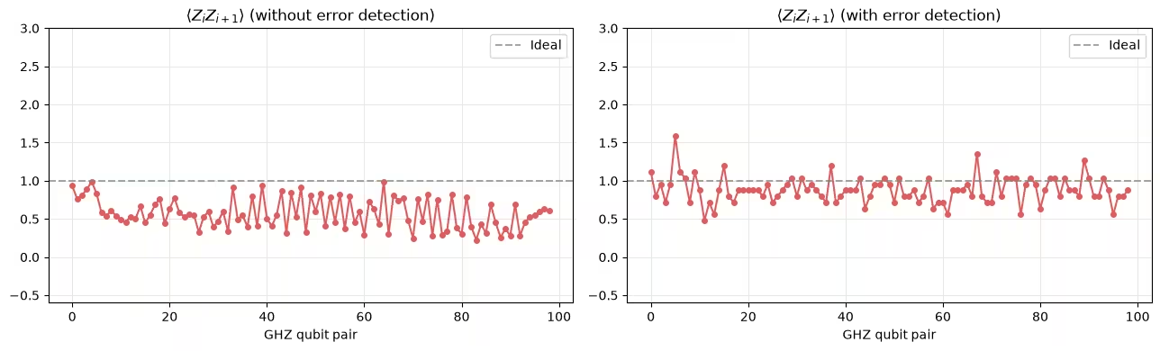
Before detection: <ZiZi+1>=  0.573749999999951
After detection: <ZiZi+1>=  0.8817377312951776

Bigyang-kahulugan ang mga resulta

Ipinapakita ng dalawang plot ang $\langle Z_i Z_{i+1}\rangle$ na tinantiya mula sa shadow tomography para sa bawat magkatabing pares ng qubit sa 100-qubit na GHZ chain, bago at pagkatapos mag-postselect sa mga parity check.

Para sa isang ideal na GHZ state, lahat ng nearest-neighbor correlator ay katumbas ng $1$. Sa hardware, ibinababa ng noise ang mga raw na tantiya at nagdudulot ng scatter mula qubit patungong qubit. Pagkatapos ng error detection, inaalis ang mga snapshot kung saan nagkaroon ng kahit isang natutukoy na error, at ang natitirang mga tantiya ay mas lumalapit sa $1$ na may mas maliit na variance, na naaayon sa mas malinis na epektibong state.

Ang pagbuti pagkatapos ng error detection ay naaayon sa mga check na nakakakita ng totoong mga error.

Mga susunod na hakbang

Tuklasin ang mga sumusunod na resource para matuto pa:

Mga Rekomendasyon

• General formulation of quantum information
• Low-overhead error detection using spacetime codes tutorial
• Qiskit Paulice add-on API documentation

Mga Sanggunian

• [1] Huang, H. Y., Kueng, R., & Preskill, J. (2020). Predicting many properties of a quantum system from very few measurements. Nature Physics, 16, 1050–1057.

• [2] Zhao, A., Rubin, N. C., & Miyake, A. (2021). Fermionic partial tomography via classical shadows. Phys. Rev. Lett., 127, 110504.

• [3] Low, G. H. (2022). Classical shadows of fermions with particle number symmetry. arXiv:2208.08964.

• [4] Bertoni, C., Haferkamp, J., Hinsche, M. et al. (2024). Shallow Shadows: Expectation Estimation Using Low-Depth Random Clifford Circuits. Phys. Rev. Lett., 133, 020602.

• [5] Hu, H.-Y., Gu, A., Majumder, S. et al. (2025). Demonstration of robust and efficient quantum property learning with shallow shadows. Nature Communications, 16, 2943.

• [6] Martiel, S. & Javadi-Abhari, A. (2025). Low-overhead error detection with spacetime codes. arXiv:2504.15725. © IBM Corp. 2026