I-simulate ang time evolution ng transverse-field Ising model
Tantiya sa paggamit: 105 segundo sa isang Nighthawk r2 processor (TANDAAN: Tantiya lang ito. Maaaring iba ang runtime mo.)
Mga learning outcome
-
Matutunan kung paano mag-transpile at magpatakbo ng mga quantum circuit sa hardware gamit ang Julia
-
Matutunan kung paano i-post-process ang mga resulta ng pagsukat para kalkulahin ang mga expectation value
-
Matutunan kung paano i-benchmark ang mga resulta ng hardware laban sa classical simulation para masukat ang pinagsamang epekto ng Trotter approximation error at hardware noise
Mga paunang kinakailangan
Maging pamilyar sa mga sumusunod na paksa bago simulan ang tutorial na ito:
Background
Ang Julia ay isang dynamic na programming language na pangunahing dinisenyo para sa numerical at scientific computing. Dahil sa mataas nitong performance sa numerical computing, natural itong akma sa mga workflow ng quantum simulation. Sa tutorial na ito, ipinapakita namin kung paano ginagamit ang Julia kapwa para sa classical na pre- at post-processing (halimbawa, pagbuo ng mga Hamiltonian, pagpapatakbo ng mga ODE (ordinary differential equation) solver, at pagkalkula ng mga expectation value) at para sa pag-orchestrate ng mga quantum hardware job, na inaalis ang pangangailangang magpalipat-lipat sa pagitan ng mga wika o environment.
Para makipag-interface sa IBM Quantum® hardware mula sa Julia, gumagamit ang tutorial na ito ng dalawang package mula sa Qiskit ecosystem: ang Qiskit.jl ay bumabalot sa Qiskit C library at nagbibigay ng circuit construction at transpilation functionality sa Julia; ang QiskitIBMRuntime.jl ay kumokonekta sa IBM Quantum hardware sa pamamagitan ng IBM Quantum Compute Service client, na nagbibigay-daan sa job submission at result retrieval nang direkta mula sa Julia.
Sa tutorial na ito, isinasaalang-alang natin ang trotterized na evolution ng transverse-field Ising model sa isang 1D chain na may nearest-neighbor na mga interaksyon:
Para ipatupad ang time evolution na , hinahati natin ang time interval na sa na hakbang at dinedefine ang . Ang second-order na Trotter-Suzuki decomposition ay nagbibigay ng sumusunod:
Para sa pagbuo ng circuit, ang bawat Trotter step ay ipinatutupad bilang sunod-sunod na single-qubit rotations at two-qubit gates. Nagsisimula ang circuit sa paghahanda ng Néel state gamit ang X gates sa magkakahalinhinang qubit. Ang bawat sumusunod na Trotter step ay naglalapat ng: (1) sa bawat qubit, (2) sa bawat magkatabing pares sa kahabaan ng chain, at (3) ulit sa bawat qubit. Ang kabuuang circuit depth ay lumalaki nang linear kasabay ng bilang ng mga Trotter step .
Mga Kinakailangan
Tandaan na kailangan ng tutorial na ito ang macOS o Linux. Hindi pa sinusuportahan ang Qiskit.jl sa Windows (sinusubaybayan sa bukas na issue na ito).
Para makapagsimula, i-install ang Julia ayon sa mga tagubilin sa pahina ng pag-download ng Julia. Binuo ang tutorial na ito gamit ang Julia 1.11; i-install ito gamit ang juliaup add 1.11.
Susunod, patakbuhin ang sumusunod na command sa isang terminal para i-install ang Julia package na IJulia sa global environment, para mapatakbo mo ang Julia sa loob ng Jupyter notebook.
julia -e 'using Pkg; Pkg.add("IJulia")'
Ginagamit natin ang built-in package manager ng Julia para i-set up ang project environment. May dalawang paraan para i-set up ang environment.
Opsyon 1: pansamantalang environment. Maaari mong patakbuhin ang sumusunod na code cell para mag-set up ng pansamantalang environment at i-install ang mga kinakailangang package;
Opsyon 2: ulitin ang eksaktong nasubukang environment. Itakda ang download_toml_files = true sa cell sa ibaba. Ida-download ng cell ang Project.toml at Manifest.toml mula sa repository ng dokumentasyon papunta sa folder na env_tutorial/time-evolution/ sa tabi ng notebook na ito, pagkatapos ay ia-activate ang environment na iyon at i-install ang eksaktong mga bersyon ng package na nakatala rito. Inilalarawan ng project file ang environment sa mataas na antas, halimbawa, inililista ng seksyong [deps] ang lahat ng dependency. Ipinapako naman ng manifest file ang eksaktong bersyon ng bawat package (kasama ang mga di-direktang dependency), kaya nauulit nang pareho ang environment. Tingnan ang dokumentasyon ng Julia para sa karagdagang detalye.
Ang mga sumusunod na dependency ay ii-install sa environment.
Para sa pagbuo at pagpapatakbo ng quantum circuit:
Qiskit.jlQiskitIBMRuntime.jl
Para sa classical simulation:
OrdinaryDiffEq.jlTensorNetworkQuantumSimulator.jl
Para sa post-processing ng mga resulta at visualization:
StatsBase.jlPlots.jl
Sinubukan ang tutorial na ito gamit ang Qiskit.jl bersyon 0.6.0 at QiskitIBMRuntime.jl bersyon 0.3.1.
using Pkg
using Downloads

download_toml_files = false

if !download_toml_files
    # Option 1: Install the latest versions of the required packages into a temporary environment
    Pkg.activate(mktempdir(); io=devnull)
    Pkg.add([
        PackageSpec(name="Qiskit"),
        PackageSpec(name="QiskitIBMRuntime"),
        PackageSpec(name="Python_jll"),
        PackageSpec(name="OrdinaryDiffEq"),
        PackageSpec(name="TensorNetworkQuantumSimulator"),
        PackageSpec(name="StatsBase"),
        PackageSpec(name="Plots"),
    ]; io=devnull)
else
    # Option 2: Install the exact tested versions pinned in the downloaded Project.toml and Manifest.toml
    base_url = "https://raw.githubusercontent.com/Qiskit/documentation/main/docs/tutorials/assets/time-evolution/julia"
    env_dir = joinpath(@__DIR__, "env_tutorial", "time-evolution")
    mkpath(env_dir)
    for file in ("Project.toml", "Manifest.toml")
        Downloads.download("$base_url/$file", joinpath(env_dir, file))
    end

    Pkg.activate(env_dir; io=devnull)
    Pkg.instantiate(; io=devnull) # installs the exact versions recorded in Manifest.toml
end
Hanggang dito, na-set up na natin ang Julia project environment para patakbuhin ang notebook. Para mapatakbo ang workflow sa isang IBM® quantum processing unit, kailangan mo ng IBM Quantum account at API token para i-instantiate ang service mula sa qiskit-ibm-runtime. Sundin ang mga hakbang na "Install and authenticate" sa paksang Run your first circuit on hardware para buuin ang iyong API token at hanapin ang iyong instance CRN.
Setup
using Qiskit
using Qiskit.Operations
using QiskitIBMRuntime
using StatsBase
using OrdinaryDiffEq
using SparseArrays
using LinearAlgebra
using TensorNetworkQuantumSimulator
using Plots: plot, plot!, heatmap, @layout, mm
Nagtatakda rin tayo ng sumusunod na utility function, na nagbabalik ng halaga ng bit sa isang bitstring na v sa posisyong i. Halimbawa, kung v = 6 (binary 110),
- ang
bit_at(6, 1)ay nagbabalik ng0, - ang
bit_at(6, 2)ay nagbabalik ng1, - ang
bit_at(6, 3)ay nagbabalik ng1.
Sinusunod nito ang little-endian convention na ginagamit sa Qiskit: ang posisyong i ay iniindex mula sa least-significant (ang "pinakakanang") bit.
"""
    bit_at(v::Integer, i::Integer) = (v >> (i-1)) & 1

Return the value of the bit at position `i` in `v`.
"""
bit_at(v::Integer, i::Integer) = (v >> (i-1)) & 1
bit_at
Halimbawa ng maliit na simulator
Isinasaalang-alang natin ang 1D chain ng qubit, na inilalarawan ng transverse-field Ising model sa itaas. Para sa sistemang pinag-aaralan, tinutukoy natin sa ibaba ang laki ng sistema na N, ang laki ng Trotter step na δt, at ang kabuuang bilang ng mga Trotter step na r_max. Ang kabuuang oras ng ebolusyon ay δt * r_max. Tandaan na sinusuportahan ng Julia ang mga Unicode identifier tulad ng δt; sa notebook o Julia REPL, i-type ang \delta na sinusundan ng Tab para mailagay ang δ. Para sa buong sanggunian, tingnan ang dokumentasyon ng Julia Unicode input.
Eksaktong solusyon
Para makagawa ng baseline na maihahambing sa mga resulta mula sa quantum hardware, ipinapakita muna natin ang classical simulation workflow para sa maliit na problema. Binubuo natin ang Ising Hamiltonian bilang sparse matrix, pagkatapos ay kinukuha ang eksaktong time evolution sa pamamagitan ng numerical na pag-integrate ng Schrödinger equation gamit ang ODEProblem mula sa OrdinaryDiffEq.jl. Ang pamamaraang ito ay lumalaki nang exponential sa bilang ng mga qubit na . Kailangan nitong itabi ang buong -dimensional na state vector. Para sa , mahigit isang milyon na ang dimensyon ng Hilbert space, kaya hindi ito praktikal para sa mas malalaking sistema.
N = 20
δt = 0.05 # Trotter step size
r_max = 10 # total number of Trotter steps

h = fill(1.0, N)
J = fill(1.0, N-1)

# Build the Ising Hamiltonian as a sparse 2^n × 2^n matrix
function build_ising_hamiltonian(h::AbstractVector{<:Real}, J::AbstractVector{<:Real}, n::Int)
    dim = 2^n

    # diagonal ZZ terms
    diag_terms = zeros(Float64, dim)
    for i in 1:n-1
        for b in 0:dim-1
            bi = bit_at(b, i) # bit at position i
            bi_next = bit_at(b, i+1) # bit at position i + 1
            diag_terms[b+1] += J[i] * (1-2bi) * (1-2bi_next)
        end
    end
    H = spdiagm(0 => complex(diag_terms))

    # off-diagonal local X terms
    for i in 1:n
        mask = 1 << (i-1)
        cols = [xor(b, mask) + 1 for b in 0:dim-1]
        H += h[i] * sparse(1:dim, cols, ones(ComplexF64, dim), dim, dim)
    end
    return H
end

H_ising = build_ising_hamiltonian(h, J, N)
1048576×1048576 SparseMatrixCSC{ComplexF64, Int64} with 22020096 stored entries:
⎡⣿⣿⣾⢦⡀⠳⣄⠀⠀⠀⠳⣄⠀⠀⠀⠀⠀⠀⠀⠀⠳⣄⠀⠀⠀⠀⠀⠀⠀⠀⠀⠀⠀⠀⠀⠀⠀⠀⠀⠀⎤
⎢⠺⣟⢻⣶⣿⡂⠈⠳⣄⠀⠀⠈⠳⣄⠀⠀⠀⠀⠀⠀⠀⠈⠳⣄⠀⠀⠀⠀⠀⠀⠀⠀⠀⠀⠀⠀⠀⠀⠀⠀⎥
⎢⢤⡈⠻⠻⠿⣧⣤⣠⡈⠳⠄⠀⠀⠈⠳⣄⠀⠀⠀⠀⠀⠀⠀⠈⠳⣄⠀⠀⠀⠀⠀⠀⠀⠀⠀⠀⠀⠀⠀⠀⎥
⎢⠀⠙⢦⡀⠀⣻⣿⣿⣙⣦⡀⠀⠀⠀⠀⠈⠳⣄⠀⠀⠀⠀⠀⠀⠀⠈⠳⣄⠀⠀⠀⠀⠀⠀⠀⠀⠀⠀⠀⠀⎥
⎢⠀⠀⠀⠙⢦⡈⠳⣼⣿⣿⡆⠀⠀⠀⠀⠀⠀⠈⠳⣄⠀⠀⠀⠀⠀⠀⠀⠈⠳⣄⠀⠀⠀⠀⠀⠀⠀⠀⠀⠀⎥
⎢⠙⢦⡀⠀⠀⠁⠀⠈⠈⠉⣿⣿⣾⢦⡀⠳⣄⠀⠀⠈⠀⠀⠀⠀⠀⠀⠀⠀⠀⠈⠳⣄⠀⠀⠀⠀⠀⠀⠀⠀⎥
⎢⠀⠀⠙⢦⡀⠀⠀⠀⠀⠀⠺⣟⢻⣶⣿⡂⠈⠳⣄⠀⠀⠀⠀⠀⠀⠀⠀⠀⠀⠀⠀⠈⠳⣄⠀⠀⠀⠀⠀⠀⎥
⎢⠀⠀⠀⠀⠙⢦⡀⠀⠀⠀⢤⡈⠻⠻⠿⣧⣤⣠⡈⠳⠀⠀⠀⠀⠀⠀⠀⠀⠀⠀⠀⠀⠀⠈⠳⣄⠀⠀⠀⠀⎥
⎢⠀⠀⠀⠀⠀⠀⠙⢦⡀⠀⠀⠙⢦⡀⠀⣻⣿⣿⣙⣦⠀⠀⠀⠀⠀⠀⠀⠀⠀⠀⠀⠀⠀⠀⠀⠈⠳⣄⠀⠀⎥
⎢⠀⠀⠀⠀⠀⠀⠀⠀⠙⢦⡀⠀⠀⠙⢦⡈⠳⣼⣿⣿⠀⠀⠀⠀⠀⠀⠀⠀⠀⠀⠀⠀⠀⠀⠀⠀⠀⠈⠳⣄⎥
⎢⠙⢦⡀⠀⠀⠀⠀⠀⠀⠀⠀⠀⠀⠀⠀⠀⠀⠀⠀⠀⣿⣿⡟⢦⡈⠳⣄⠀⠀⠈⠳⣄⠀⠀⠀⠀⠀⠀⠀⠀⎥
⎢⠀⠀⠙⢦⡀⠀⠀⠀⠀⠀⠀⠀⠀⠀⠀⠀⠀⠀⠀⠀⠻⣍⣿⣿⣯⠀⠈⠳⣄⠀⠀⠈⠳⣄⠀⠀⠀⠀⠀⠀⎥
⎢⠀⠀⠀⠀⠙⢦⡀⠀⠀⠀⠀⠀⠀⠀⠀⠀⠀⠀⠀⠀⢦⡈⠋⠛⢻⣶⣦⣦⡈⠓⠀⠀⠀⠈⠳⣄⠀⠀⠀⠀⎥
⎢⠀⠀⠀⠀⠀⠀⠙⢦⡀⠀⠀⠀⠀⠀⠀⠀⠀⠀⠀⠀⠀⠙⢦⡀⠨⣿⠿⣧⣽⡦⠀⠀⠀⠀⠀⠈⠳⣄⠀⠀⎥
⎢⠀⠀⠀⠀⠀⠀⠀⠀⠙⢦⡀⠀⠀⠀⠀⠀⠀⠀⠀⠀⡀⠀⠀⠙⢦⠈⠳⡿⣿⣿⣀⡀⡀⠀⢀⠀⠀⠈⠳⣄⎥
⎢⠀⠀⠀⠀⠀⠀⠀⠀⠀⠀⠙⢦⡀⠀⠀⠀⠀⠀⠀⠀⠙⢦⡀⠀⠀⠀⠀⠀⠀⠸⣿⣿⡟⢦⡈⠳⣄⠀⠀⠀⎥
⎢⠀⠀⠀⠀⠀⠀⠀⠀⠀⠀⠀⠀⠙⢦⡀⠀⠀⠀⠀⠀⠀⠀⠙⢦⡀⠀⠀⠀⠀⠈⠻⣍⣿⣿⣯⠀⠈⠳⣄⠀⎥
⎢⠀⠀⠀⠀⠀⠀⠀⠀⠀⠀⠀⠀⠀⠀⠙⢦⡀⠀⠀⠀⠀⠀⠀⠀⠙⢦⡀⠀⠀⠐⢦⡈⠋⠛⢻⣶⣦⣦⡈⠓⎥
⎢⠀⠀⠀⠀⠀⠀⠀⠀⠀⠀⠀⠀⠀⠀⠀⠀⠙⢦⡀⠀⠀⠀⠀⠀⠀⠀⠙⢦⡀⠀⠀⠙⢦⡀⠨⣿⠿⣧⣽⡦⎥
⎣⠀⠀⠀⠀⠀⠀⠀⠀⠀⠀⠀⠀⠀⠀⠀⠀⠀⠀⠙⢦⠀⠀⠀⠀⠀⠀⠀⠀⠙⢦⠀⠀⠀⠙⢦⠈⠳⡿⣿⣿⎦
Itinatakda natin ang kanang bahagi ng Schrödinger equation sa in-place na anyong schrodinger!(dψ, ψ, H, t), na kumukwenta ng gamit ang sparse matrix-vector multiplication. Pagkatapos ay nagse-set up tayo ng ODEProblem na may Néel state bilang paunang kondisyon at nilulutas ito sa saklaw ng oras na , na sine-save ang state sa bawat time step na . Ang ginamit na solver ay Tsit5(), isang karaniwang explicit na fourth/fifth-order Runge-Kutta method na angkop para sa mga non-stiff na problema.
# initial state |0101...01⟩
ψ0 = zeros(ComplexF64, 2^N)
neel_index = sum(1 << (i-1) for i in 1:2:N)
ψ0[neel_index + 1] = 1.0

function schrodinger!(dψ::AbstractVector, ψ::AbstractVector, H::AbstractMatrix, t::Real)
    mul!(dψ, H, ψ)
    dψ .*= -im
end

tspan = (0.0, r_max * δt)
prob = ODEProblem(schrodinger!, ψ0, tspan, H_ising)
sol = solve(prob, Tsit5(), saveat=δt)
retcode: Success
Interpolation: 1st order linear
t: 11-element Vector{Float64}:
 0.0
 0.05
 0.1
 0.15
 0.2
 0.25
 0.3
 0.35
 0.4
 0.45
 0.5
u: 11-element Vector{Vector{ComplexF64}}:
 [0.0 + 0.0im, 0.0 + 0.0im, 0.0 + 0.0im, 0.0 + 0.0im, 0.0 + 0.0im, 0.0 + 0.0im, 0.0 + 0.0im, 0.0 + 0.0im, 0.0 + 0.0im, 0.0 + 0.0im  …  0.0 + 0.0im, 0.0 + 0.0im, 0.0 + 0.0im, 0.0 + 0.0im, 0.0 + 0.0im, 0.0 + 0.0im, 0.0 + 0.0im, 0.0 + 0.0im, 0.0 + 0.0im, 0.0 + 0.0im]
 [-7.612535273941705e-14 + 2.5737401150886516e-29im, 7.616818423232204e-14 - 1.6944517510822304e-12im, -8.565903349044157e-17 + 3.2368190823993794e-15im, -7.61682079584434e-14 - 1.078515326911689e-15im, 1.523363843119942e-13 - 1.6912125988569567e-12im, 3.5867824743714624e-11 + 5.083352813839524e-12im, -7.608249752495255e-14 - 4.317561743447096e-15im, 7.616820798431766e-14 - 1.6944516451719627e-12im, -8.570258514925147e-17 + 3.2384113624188233e-15im, -7.606534127496737e-14 - 5.398093819616815e-15im  …  -7.591102113501652e-14 - 7.55501666902211e-15im, 1.5233640806402347e-13 - 1.691212597789024e-12im, -4.283149391646935e-17 + 3.2390475588024777e-15im, -7.61253567131055e-14 - 4.319154099332238e-15im, 1.28498500555455e-16 + 4.773388002812907e-18im, -8.570258413862945e-17 + 3.2384113624488572e-15im, -7.612534879063769e-14 - 3.2390464923709225e-15im, 1.5233638826330585e-13 - 1.6912127047672224e-12im, -4.283149290692347e-17 + 3.237455101084436e-15im, -7.612535273941595e-14 - 1.8338992189508272e-31im]
 [-8.680854672628291e-11 - 3.427254579020333e-25im, 8.709110140864061e-11 - 8.699033104505336e-10im, -5.649235901782656e-13 + 8.601572275260816e-12im, -8.709221846767839e-11 - 2.859732693854631e-12im, 1.7418295344900034e-10 - 8.612608133903897e-10im, 8.41248317362033e-9 + 2.6096671235273274e-9im, -8.652487588621059e-11 - 1.1500395899126693e-11im, 8.709222358844944e-11 - 8.699014655672987e-10im, -5.669821718119223e-13 + 8.629638578162805e-12im, -8.641073444337035e-11 - 1.4395664161950265e-11im  …  -8.538755211456945e-11 - 2.0113079067784756e-11im, 1.7418407565004836e-10 - 8.612606969068827e-10im, -2.825548799186401e-13 + 8.640787361594646e-12im, -8.680873675466659e-11 - 1.152847038256832e-11im, 8.478635815548866e-13 + 8.382372443494577e-14im, -5.669819735592012e-13 + 8.629638588149376e-12im, -8.680836165042751e-11 - 8.640671375786309e-12im, 1.7418313902498964e-10 - 8.61262658275938e-10im, -2.82554682353394e-13 + 8.612701741862262e-12im, -8.680854672628374e-11 - 2.811149115586865e-25im]
 [-4.2861942928308275e-9 - 4.7678984538985196e-24im, 4.318192995176613e-9 - 2.8269371315624182e-8im, -6.395173522788358e-11 + 6.447233357075582e-10im, -4.318468070877377e-9 - 2.1364257686596578e-10im, 8.636571975410676e-9 - 2.7617721500979347e-8im, 1.7289660717976908e-7 + 8.480086489483005e-8im, -4.253920910159066e-9 - 8.649865429907717e-10im, 4.318470318624579e-9 - 2.826906169988642e-8im, -6.446071076018044e-11 + 6.495016281145607e-10im, -4.240844230135151e-9 - 1.0846764703342651e-9im  …  -4.124170626784771e-9 - 1.5115818225612714e-9im, 8.636849310525618e-9 - 2.7617681592276622e-8im, -3.199878870600196e-11 + 6.513863923787342e-10im, -4.2862418335791054e-9 - 8.697676141630365e-10im, 9.60478168658149e-11 + 1.4206678132640617e-11im, -6.446062402203318e-11 + 6.495016332435747e-10im, -4.286148929585427e-9 - 6.513467397401749e-10im, 8.636617557977306e-9 - 2.7618031117900408e-8im, -3.1998702345812497e-11 + 6.466014984949206e-10im, -4.286194292830829e-9 + 4.870909626742163e-24im]
 [-6.079348924748445e-8 + 6.709717322272516e-24im, 6.162943323939352e-8 - 2.9592110353110093e-7im, -1.6696556398383817e-9 + 1.2400459826013194e-8im, -6.164292787255694e-8 - 4.088131560944853e-9im, 1.2326810978249792e-7 - 2.832733452226872e-7im, 1.253532043962043e-6 + 8.875042569125039e-7im, -5.994408800994472e-8 - 1.6725258647088304e-8im, 6.164314112979357e-8 - 2.9591021577421156e-7im, -1.6948387141108349e-9 + 1.2572865374243683e-8im, -5.959595610442699e-8 - 2.1031419496566967e-8im  …  -5.651357562833814e-8 - 2.9192023780832225e-8im, 1.2328181992163385e-7 - 2.832706038202527e-7im, -8.359520177503641e-10 + 1.2640019589288568e-8im, -6.079590106381668e-8 - 1.689785040734888e-8im, 2.5106376181130386e-9 + 5.084778396177926e-10im, -1.6948306165735295e-9 + 1.2572866042727832e-8im, -6.079128573701664e-8 - 1.2637312624047932e-8im, 1.2327033399936622e-7 - 2.8328423313378375e-7im, -8.359439919088748e-10 + 1.2467163914771088e-8im, -6.079348924748447e-8 + 1.0331673240130025e-23im]
 [-4.193552407608965e-7 - 1.840220498495959e-23im, 4.2862657866184504e-7 - 1.605297190776032e-6im, -1.8502762435969943e-8 + 1.0856276308591437e-7im, -4.288690355597115e-7 - 3.554458373697522e-8im, 8.574220964863143e-7 - 1.4932465582703908e-6im, 4.849187224415274e-6 + 4.812233679729101e-6im, -4.098425461298137e-7 - 1.4745065418194435e-7im, 4.288753395920834e-7 - 1.6051467128773302e-6im, -1.896035285782807e-8 + 1.1102835700521827e-7im, -4.0588320553359593e-7 - 1.8611022850670223e-7im  …  -3.711838427223188e-7 - 2.569391306045151e-7im, 8.57670971098675e-7 - 1.4931825847645462e-6im, -9.271568570757063e-9 + 1.1197289579952942e-7im, -4.194005371452928e-7 - 1.4992045110994755e-7im, 2.787088237718031e-8 + 7.194933454521717e-9im, -1.8960118645415406e-8 + 1.1102838165568638e-7im, -4.193161709409199e-7 - 1.1191024844294344e-7im, 8.574617742181924e-7 - 1.4933970418540967e-6im, -9.271337900947239e-9 + 1.0949690324053836e-7im, -4.193552407608964e-7 + 1.6524848989693985e-22im]
 [-1.7823579016922897e-6 - 1.087640585040274e-21im, 1.840838369770109e-6 - 5.569854913729441e-6im, -1.1658899308162594e-7 + 5.632670364049069e-7im, -1.843111911436975e-6 - 1.8277839588324167e-7im, 3.6832950716080163e-6 - 4.979757871286645e-6im, 1.1823232043972897e-5 + 1.668138856075027e-5im, -1.7216192586061922e-6 - 7.718155525067347e-7im, 1.8432004842500001e-6 - 5.56872697042903e-6im, -1.209408931510706e-7 + 5.825677201706816e-7im, -1.6958321412209815e-6 - 9.789484717969276e-7im  …  -1.4727630743780977e-6 - 1.3421173522554028e-6im, 3.6856596566327488e-6 - 4.9790105233659736e-6im, -5.848359517965976e-8 + 5.898080282235565e-7im, -1.7828068643880377e-6 - 7.911632992433939e-7im, 1.760517112427114e-7 + 5.557422909554899e-8im, -1.209376913040035e-7 + 5.825681268981909e-7im, -1.7819976541714096e-6 - 5.890838036292954e-7im, 3.6836637838442504e-6 - 4.980885908360778e-6im, -5.848046807781978e-8 + 5.703874412047737e-7im, -1.7823579016922876e-6 + 1.4997773495573015e-22im]
 [-5.2719847869895295e-6 + 8.772351797140282e-21im, 5.515796864069832e-6 - 1.3769890958036113e-5im, -4.854583030811284e-7 + 1.984102714841576e-6im, -5.52914007682216e-6 - 6.365426377065764e-7im, 1.1041341496086288e-5 - 1.1652942788167796e-5im, 1.9151485012220565e-5 + 4.1169949873337434e-5im, -5.0149560721693026e-6 - 2.748560607544284e-6im, 5.529875137426081e-6 - 1.3764484293927507e-5im, -5.114444270677655e-7 + 2.0817439894898367e-6im, -4.903067916522327e-6 - 3.508133202204623e-6im  …  -3.950715241692067e-6 - 4.767013437270117e-6im, 1.1055449702075777e-5 - 1.1647607717886785e-5im, -2.4383689790869913e-7 + 2.1174362562762014e-6im, -5.274804158840664e-6 - 2.846520575369006e-6im, 7.355815857851513e-7 + 2.7656731682993024e-7im, -5.114187341304747e-7 + 2.0817477909234415e-6im, -5.2699143882793144e-6 - 2.112332735357189e-6im, 1.1043481329588082e-5 - 1.1658350328429614e-5im, -2.438120770802614e-7 + 2.018953103020384e-6im, -5.271984786989539e-6 + 6.138686657683503e-21im]
 [-1.1617825704147756e-5 + 1.0312565819538484e-21im, 1.2349337633136464e-5 - 2.5744303624623147e-5im, -1.454293291805138e-6 + 5.123664098726546e-6im, -1.2403650700016836e-5 - 1.6202581807656819e-6im, 2.473960492472325e-5 - 2.0155561130978555e-5im, 1.9144096039811722e-5 + 7.6742969783544e-5im, -1.0832694804431494e-5 - 7.1930875309620025e-6im, 1.2407719644833958e-5 - 2.572612053989065e-5im, -1.56229208977908e-6 + 5.474515092672054e-6im, -1.0480130191816845e-5 - 9.254685626031852e-6im  …  -7.537537188446326e-6 - 1.2435206581306264e-5im, 2.4798220145598703e-5 - 2.0129513964044365e-5im, -7.316420138432232e-7 + 5.598791194770797e-6im, -1.1630271281791021e-5 - 7.545396775206743e-6im, 2.2142322134173096e-6 + 9.742099793903422e-7im, -1.5621555243617513e-6 + 5.474538012007301e-6im, -1.1609612670484607e-5 - 5.574263610620754e-6im, 2.4748196626943606e-5 - 2.0173749496261283e-5im, -7.315119289888009e-7 + 5.243914596674148e-6im, -1.1617825704147746e-5 + 2.0077178062353968e-21im]
 [-1.9812558848038747e-5 - 9.187798066332235e-22im, 2.147271081932555e-5 - 3.757217609507472e-5im, -3.2943974661872274e-6 + 1.0138423201098428e-5im, -2.163583224409355e-5 - 3.1479593611068202e-6im, 4.3072956212126986e-5 - 2.6216146005671797e-5im, 4.770433131249609e-6 + 0.00011143181451766211im, -1.7992013464296718e-5 - 1.4466566267165694e-5im, 2.1652013724844488e-5 - 3.752687773861608e-5im, -3.6269134427165884e-6 + 1.1086241359275966e-5im, -1.7142579310500252e-5 - 1.8804566182208357e-5im  …  -1.0216935244391546e-5 - 2.491043927093904e-5im, 4.325353440439837e-5 - 2.6122963951736878e-5im, -1.6606359562313976e-6 + 1.140941830342574e-5im, -1.9853711381944784e-5 - 1.541920404485947e-5im, 5.050007317756615e-6 + 2.569541043839736e-6im, -3.6263960453836696e-6 + 1.1086337766500889e-5im, -1.97886585017898e-5 - 1.1323323936752868e-5im, 4.309833408283902e-5 - 2.6261466566058982e-5im, -1.6601519712867477e-6 + 1.044756873253024e-5im, -1.981255884803875e-5 + 7.339651656276922e-20im]
 [-2.6605994524636198e-5 + 1.1289591858171765e-19im, 2.9532145628332138e-5 - 4.333877076489454e-5im, -5.793688435837011e-6 + 1.572023652812328e-5im, -2.9906819721527362e-5 - 4.767746092973603e-6im, 5.9370303731772103e-5 - 2.51584831603933e-5im, -2.1873141629015348e-5 + 0.00012741720406900944im, -2.3313208885217603e-5 - 2.288272975975095e-5im, 2.995521974547466e-5 - 4.325274969426522e-5im, -6.580507052690018e-6 + 1.770923159800008e-5im, -2.1702668886267368e-5 - 3.0142728729320425e-5im  …  -8.927183090969304e-6 - 3.921197964153728e-5im, 5.979856139686108e-5 - 2.4903653161242186e-5im, -2.9274853045629046e-6 + 1.8356702741523666e-5im, -2.6711940545518465e-5 - 2.488368314305582e-5im, 8.967724203429812e-6 + 5.238269352768273e-6im, -6.579046665900031e-6 + 1.770952822000892e-5im, -2.6553193423229552e-5 - 1.812661956307733e-5im, 5.942741740138485e-5 - 2.5244572524328294e-5im, -2.9261511036959703e-6 + 1.6330572728121542e-5im, -2.660599452463617e-5 - 3.440870688152987e-20im]
Mula sa solusyon, na naglalarawan sa state vector na , makukuha natin ang magnetization kada site, na ipinapahayag bilang mga single-qubit expectation value bilang function ng oras. Ihahambing natin ito sa mga resultang nakuha mula sa mga Trotterized circuit.
# get a single-qubit expectation value ⟨Z_qubit⟩ from a full state vector, weighting ±1 by |amplitude|²
function z_expval_from_state(ψ::AbstractVector{<:Complex}, qubit::Int, n::Int)
    s = 0.0
    for b in 0:2^n-1
        bit = bit_at(b, qubit)
        s += (1 - 2bit) * abs2(ψ[b+1])
    end
    return s
end

classical_magnetizations = [z_expval_from_state(sol.u[r+1], q, N)
                             for r in 0:r_max, q in 1:N]
11×20 Matrix{Float64}:
 -1.0       1.0       -1.0       1.0       …  1.0       -1.0       1.0
 -0.995021  0.995034  -0.995034  0.995034     0.995034  -0.995034  0.995021
 -0.980189  0.980386  -0.980386  0.980386     0.980386  -0.980386  0.980189
 -0.955994  0.956968  -0.956968  0.956968     0.956968  -0.956968  0.955994
 -0.922667  0.925652  -0.925653  0.925653     0.925653  -0.925652  0.922667
 -0.881106  0.888117  -0.88812   0.88812   …  0.88812   -0.888117  0.881106
 -0.832251  0.846116  -0.846129  0.846129     0.846129  -0.846116  0.832251
 -0.776957  0.801257  -0.801298  0.801298     0.801298  -0.801257  0.776957
 -0.715858  0.754749  -0.75486   0.75486      0.75486   -0.754749  0.715858
 -0.649744  0.707628  -0.707895  0.707895     0.707895  -0.707628  0.649744
 -0.580117  0.661272  -0.661841  0.661842  …  0.661841  -0.661272  0.580117
Maliit na simulation ng mga Trotterized circuit
Sa sumusunod, ipinapakita natin ang classical simulation ng mga noiseless circuit gamit ang mga tensor network method na sinusuportahan ng TensorNetworkQuantumSimulator.jl, para ma-validate natin ang pagbuo ng ating circuit. Nagbibigay ang mga method na ito ng baseline na maihahambing sa mga resulta mula sa quantum hardware.
Una nating itinatakda ang lattice bilang 1D chain graph gamit ang named_grid((N,)), kung saan ang bawat vertex ay isang tuple na (i,). Pagkatapos ay tinutukoy natin ang mga circuit gate bilang listahan ng mga tuple na (gate_name, qubit_indices, gate_parameter), na nagsisilbing input format para sa tensor network simulator.
# 1D chain graph — vertices are named (1,), (2,), ..., (N,)
g = named_grid((N,))

# Gates to prepare Néel state |0101…⟩, X on every other site
neel_state_gates(n::Int) = [("X", [(i,)]) for i in 1:2:n]

# Gates for one second-order Trotter step of size δt
trotter_step_gates(h::AbstractVector{<:Real}, J::AbstractVector{<:Real}, n::Int, δt::Real) = vcat(
    [("Rx",  [(i,)],         h[i] * δt) for i in 1:n],
    [("Rzz", [(i,), (i+1,)], 2 * J[i] * δt) for i in 1:n-1],
    [("Rx",  [(i,)],         h[i] * δt) for i in 1:n])

# Make a list of gates: Néel state preparation followed by n_trotter_steps Trotter steps
function make_trotter_circuit_tn(h::AbstractVector{<:Real}, J::AbstractVector{<:Real}, n::Int, δt::Real,
                                 n_trotter_steps::Int)
    circuit = []

    # Neel state initialization
    append!(circuit, neel_state_gates(n))

    for _ in 1:n_trotter_steps
        append!(circuit, trotter_step_gates(h, J, n, δt))
    end

    return circuit
end
make_trotter_circuit_tn (generic function with 1 method)
Ginagamit natin ang belief propagation algorithm para sa tensor network contraction. Episyente ang method na ito para sa mga circuit na may limitadong entanglement, ngunit bumababa ang katumpakan nito habang lumalaki ang entanglement kasabay ng circuit depth. Kinokontrol ng mga parameter na maxdim at cutoff ang trade-off sa pagitan ng katumpakan at gastos sa computation. Gayundin, kinukwenta natin ang magnetization sa bawat site para maihambing mamaya.
apply_kwargs = (; maxdim=32, cutoff=1e-10, normalize_tensors=true)
tn_magnetizations = zeros(r_max+1, N)

# |↑↑…↑⟩ product state, wrapped in a belief propagation cache
tn_initial_state(g::NamedGraph) = BeliefPropagationCache(
    tensornetworkstate(ComplexF32, v -> "↑", g, "S=1/2"))

# Apply a gate list to a TN state; returns the evolved state and the
# truncation fidelity, such as ∏(1 - ε) over all gate applications
function apply_gates_to_tn_state(circuit::Vector, ψ_bpc::BeliefPropagationCache; apply_kwargs::NamedTuple)
    ψ_bpc, errs = apply_gates(circuit, ψ_bpc; apply_kwargs)
    return ψ_bpc, prod(1.0 .- errs)
end

# ⟨Z_q⟩ on every site of a tensor-network state
z_expvals_from_tn_state(ψ_bpc::BeliefPropagationCache, n::Int) =
    [real(expect(ψ_bpc, [("Z", [(q,)])])[1]) for q in 1:n]

for r in 0:r_max
    circuit = make_trotter_circuit_tn(h, J, N, δt, r)
    ψ_bpc, fidelity = apply_gates_to_tn_state(circuit, tn_initial_state(g); apply_kwargs)
    println("fidelity at Trotter step $(r) was $(fidelity)")
    tn_magnetizations[r+1, :] = z_expvals_from_tn_state(ψ_bpc, N)
end
fidelity at Trotter step 0 was 1.0
fidelity at Trotter step 1 was 1.0
fidelity at Trotter step 2 was 1.0
fidelity at Trotter step 3 was 0.9999999999999679
fidelity at Trotter step 4 was 0.9999999999976941
fidelity at Trotter step 5 was 0.9999999999476229
fidelity at Trotter step 6 was 0.9999999993741544
fidelity at Trotter step 7 was 0.9999999993647009
fidelity at Trotter step 8 was 0.9999999992323603
fidelity at Trotter step 9 was 0.9999999980892764
fidelity at Trotter step 10 was 0.9999999980892698
Hakbang 1: I-map ang mga classical input sa isang quantum na problema
Ngayon, binubuo natin ang Trotterized time-evolution circuit gamit ang Qiskit.jl. Ginagaya ng circuit ang bersyon ng tensor network: ini-initialize nito ang Néel state, naglalapat ng Trotter step ng at gates, at sa huli ay sinusukat ang lahat ng qubit sa Z basis.
function make_trotter_circuit(h::AbstractVector{<:Real}, J::AbstractVector{<:Real}, n::Int, δt::Real, n_trotter_steps::Int)
    qc = QuantumCircuit(n, n)

    # Neel state initialization
    for i in 1:2:n
        x!(qc, i)
    end

    # Trotter evolution
    for _ in 1:n_trotter_steps
        for i in 1:n
            rx!(qc, h[i] * δt, i)
        end

        for i in 1:n-1
            rzz!(qc, 2* J[i] * δt, i, i+1)
        end

        for i in 1:n
            rx!(qc, h[i] * δt, i)
        end
    end

    # measure in Z basis
    for i in 1:n
        measure!(qc, i, i)
    end
    return qc
end

qc = make_trotter_circuit(h, J, N, δt, 1)
QuantumCircuit with 20 qubits, 20 clbits
  instructions: 89
Gumagawa tayo ng listahan ng mga circuit para sa mga Trotter step na 0 hanggang 10, na tumutugma sa mga oras ng ebolusyon na .
# prepare a list of circuits with different Trotter steps
qc_list = [make_trotter_circuit(h, J, N, δt, r) for r in 0:r_max]
11-element Vector{QuantumCircuit}:
 QuantumCircuit(20, 20; 30 instructions)
 QuantumCircuit(20, 20; 89 instructions)
 QuantumCircuit(20, 20; 148 instructions)
 QuantumCircuit(20, 20; 207 instructions)
 QuantumCircuit(20, 20; 266 instructions)
 QuantumCircuit(20, 20; 325 instructions)
 QuantumCircuit(20, 20; 384 instructions)
 QuantumCircuit(20, 20; 443 instructions)
 QuantumCircuit(20, 20; 502 instructions)
 QuantumCircuit(20, 20; 561 instructions)
 QuantumCircuit(20, 20; 620 instructions)
Hakbang 2: I-optimize ang problema para sa pagpapatakbo sa quantum hardware
Para tumakbo sa quantum hardware, kailangan munang i-transpile ang mga circuit. Kasama rito ang mga sumusunod na hakbang: pumili ng set ng mga pisikal na qubit kung saan ima-map ang circuit, muling i-compile ang mga gate sa native instruction set ng backend, at i-optimize ang nagreresultang circuit depth. Ginagamit natin ang least_busy() para awtomatikong piliin ang pinakakaunting abalang available na backend, ang target_from_backend() para kunin ang native gate set at qubit connectivity nito, at ang transpile() para isagawa ang compilation.
service = Service()
search_results = backend_search(service)
backend = least_busy(search_results)
@show backend.name
backend.name = "ibm_phoenix"
"ibm_phoenix"
target = target_from_backend(backend, service)
Target with 120 qubits
  instructions: 8
tqc_list = [transpile(qc, target)[1] for qc in qc_list]
11-element Vector{QuantumCircuit}:
 QuantumCircuit(120, 20; 30 instructions)
 QuantumCircuit(120, 20; 211 instructions)
 QuantumCircuit(120, 20; 344 instructions)
 QuantumCircuit(120, 20; 475 instructions)
 QuantumCircuit(120, 20; 606 instructions)
 QuantumCircuit(120, 20; 737 instructions)
 QuantumCircuit(120, 20; 868 instructions)
 QuantumCircuit(120, 20; 999 instructions)
 QuantumCircuit(120, 20; 1130 instructions)
 QuantumCircuit(120, 20; 1261 instructions)
 QuantumCircuit(120, 20; 1392 instructions)
Pagkatapos ng transpilation, sinusuri natin ang dalawang katangian ng mga na-compile na circuit. Ibinabalik ng get_circuit_layout() ang set ng mga pisikal na qubit index na napili para sa circuit. Kinukwenta ng two_qubit_depth() ang two-qubit gate depth — ang haba ng pinakamahabang chain ng mga two-qubit operation sa circuit — na kapaki-pakinabang na indikasyon ng naiipong noise sa hardware.
function get_circuit_layout(tqc::QuantumCircuit)
    return Set(q for inst in tqc.data for q in inst.qubits)
end

get_circuit_layout(tqc_list[2])
Set{Int64} with 20 elements:
  35
  110
  58
  12
  24
  37
  23
  22
  47
  69
  36
  80
  109
  90
  57
  34
  13
  59
  70
  100
Sa ibaba, ipinapakita natin ang bilang ng two-qubit gate at ang circuit depth sa bawat Trotter step; gaya ng inaasahan, parehong lumalaki nang linear kasabay ng bilang ng mga step. Tandaan na ang fractional na gate ay hindi pa available sa pamamagitan ng C API (tingnan ang qiskit-ibm-runtime-c#29). Dahil dito, ang bawat RZZGate ay itinatranspile sa dalawang two-qubit gate sa halip na isa, na nagpapalaki sa bilang ng two-qubit gate.
two_qubit_count(qc::QuantumCircuit) = count(inst -> length(inst.qubits) == 2, qc.data)

function two_qubit_depth(qc::QuantumCircuit)
    qubit_depth = Dict{Int,Int}()
    for inst in qc.data
        length(inst.qubits) == 2 || continue   # skip non-two-qubit gates
        d = maximum(get(qubit_depth, q, 0) for q in inst.qubits)
        for q in inst.qubits
            qubit_depth[q] = d + 1
        end
    end
    return isempty(qubit_depth) ? 0 : maximum(values(qubit_depth))
end

for (i, tqc) in enumerate(tqc_list)
    println("r=$(i-1): 2q gate count=$(two_qubit_count(tqc)), 2q gate depth=$(two_qubit_depth(tqc))")
end
r=0: 2q gate count=0, 2q gate depth=0
r=1: 2q gate count=38, 2q gate depth=38
r=2: 2q gate count=76, 2q gate depth=42
r=3: 2q gate count=114, 2q gate depth=46
r=4: 2q gate count=152, 2q gate depth=50
r=5: 2q gate count=190, 2q gate depth=54
r=6: 2q gate count=228, 2q gate depth=58
r=7: 2q gate count=266, 2q gate depth=62
r=8: 2q gate count=304, 2q gate depth=66
r=9: 2q gate count=342, 2q gate depth=70
r=10: 2q gate count=380, 2q gate depth=74
Hakbang 3: Patakbuhin gamit ang mga Qiskit primitive
Ngayon, maaari na nating isumite ang mga na-transpile na circuit sa backend bilang mga Sampler job na may tinukoy na shots.
shots = 1024
job_list = [run_sampler_job(service, backend, tqc, shots) for tqc in tqc_list]
11-element Vector{QiskitIBMRuntime.Job}:
 QiskitIBMRuntime.Job(Ptr{QiskitIBMRuntime.LibQiskitIBMRuntime.Job} @0x00000003427f72f0)
 QiskitIBMRuntime.Job(Ptr{QiskitIBMRuntime.LibQiskitIBMRuntime.Job} @0x00000004b2d1b4e0)
 QiskitIBMRuntime.Job(Ptr{QiskitIBMRuntime.LibQiskitIBMRuntime.Job} @0x00000004b2dcb180)
 QiskitIBMRuntime.Job(Ptr{QiskitIBMRuntime.LibQiskitIBMRuntime.Job} @0x00000004b1e24840)
 QiskitIBMRuntime.Job(Ptr{QiskitIBMRuntime.LibQiskitIBMRuntime.Job} @0x00000004b266e640)
 QiskitIBMRuntime.Job(Ptr{QiskitIBMRuntime.LibQiskitIBMRuntime.Job} @0x00000004b2d1b690)
 QiskitIBMRuntime.Job(Ptr{QiskitIBMRuntime.LibQiskitIBMRuntime.Job} @0x0000000104c17980)
 QiskitIBMRuntime.Job(Ptr{QiskitIBMRuntime.LibQiskitIBMRuntime.Job} @0x00000004b315b9b0)
 QiskitIBMRuntime.Job(Ptr{QiskitIBMRuntime.LibQiskitIBMRuntime.Job} @0x0000000104c16090)
 QiskitIBMRuntime.Job(Ptr{QiskitIBMRuntime.LibQiskitIBMRuntime.Job} @0x0000000104c195f0)
 QiskitIBMRuntime.Job(Ptr{QiskitIBMRuntime.LibQiskitIBMRuntime.Job} @0x00000004b2d33f70)
for (i, job) in enumerate(job_list)
    status = get_job_status(job, service)
    println("Job $i: ", status)
end
Job 1: Completed
Job 2: Completed
Job 3: Completed
Job 4: Completed
Job 5: Completed
Job 6: Completed
Job 7: Completed
Job 8: Completed
Job 9: Completed
Job 10: Completed
Job 11: Completed
Habang natatapos ang mga job, makukuha natin ang kanilang mga resulta. Tandaan na hihintayin ng function na get_sampler_job_results hanggang matapos ang job.
all_samples = [get_sampler_job_results(job, service) for job in job_list]
11-element Vector{QiskitIBMRuntime.Samples}:
 [[1, 0, 1, 0, 1, 0, 1, 0, 1, 0, 1, 0, 1, 0, 1, 0, 1, 0, 1, 0], [1, 0, 1, 0, 1, 0, 1, 0, 1, 0, 1, 0, 1, 0, 1, 0, 1, 0, 1, 0], [1, 0, 1, 0, 1, 0, 1, 0, 1, 0, 1, 0, 1, 0, 1, 0, 1, 0, 1, 0], [1, 0, 1, 0, 1, 1, 1, 0, 1, 0, 1, 0, 1, 0, 1, 0, 1, 0, 1, 0], [1, 0, 1, 0, 1, 0, 1, 0, 1, 0, 1, 0, 1, 0, 1, 0, 1, 0, 1, 0], [1, 0, 1, 0, 1, 0, 1, 0, 1, 0, 1, 0, 1, 0, 1, 0, 1, 0, 1, 0], [1, 0, 1, 0, 1, 0, 1, 0, 1, 0, 1, 0, 1, 0, 1, 0, 1, 0, 1, 0], [1, 0, 1, 0, 1, 0, 1, 0, 1, 0, 1, 0, 1, 0, 1, 0, 1, 0, 1, 0], [1, 0, 1, 0, 1, 0, 1, 0, 1, 0, 1, 0, 1, 0, 1, 0, 1, 0, 1, 0], [1, 0, 1, 0, 1, 0, 1, 0, 1, 0, 1, 0, 1, 0, 1, 0, 1, 0, 1, 0]  …  [1, 0, 1, 0, 1, 0, 1, 0, 1, 0, 1, 0, 1, 0, 1, 0, 1, 0, 1, 0], [1, 0, 1, 0, 1, 0, 1, 0, 1, 0, 1, 0, 1, 0, 1, 0, 1, 0, 1, 0], [1, 0, 1, 0, 1, 0, 1, 0, 1, 0, 1, 0, 1, 0, 1, 0, 1, 0, 1, 0], [1, 0, 1, 0, 1, 0, 1, 0, 1, 0, 1, 0, 1, 0, 1, 0, 1, 0, 1, 0], [1, 0, 1, 0, 1, 0, 1, 0, 1, 0, 1, 0, 1, 0, 1, 0, 1, 0, 1, 0], [1, 0, 1, 0, 1, 0, 1, 0, 1, 0, 1, 0, 1, 0, 1, 0, 1, 0, 1, 0], [1, 0, 1, 0, 1, 0, 1, 0, 1, 0, 1, 0, 1, 0, 1, 0, 1, 0, 1, 0], [1, 0, 1, 0, 1, 0, 1, 0, 1, 0, 1, 0, 1, 0, 1, 0, 1, 0, 1, 0], [1, 0, 1, 0, 1, 0, 1, 0, 1, 0, 1, 0, 1, 0, 1, 0, 1, 0, 1, 0], [1, 0, 1, 0, 1, 0, 1, 0, 1, 0, 1, 0, 1, 0, 1, 0, 1, 0, 1, 0]]
 [[1, 0, 1, 0, 0, 0, 1, 0, 1, 0, 1, 0, 1, 0, 1, 0, 1, 1, 1, 0], [1, 0, 1, 0, 1, 0, 1, 0, 1, 0, 1, 0, 1, 0, 1, 0, 1, 0, 1, 0], [1, 0, 1, 0, 1, 0, 1, 0, 1, 0, 1, 0, 1, 0, 1, 0, 1, 0, 1, 0], [1, 0, 1, 0, 1, 0, 1, 0, 1, 0, 1, 0, 1, 0, 0, 0, 1, 0, 1, 0], [1, 0, 1, 0, 1, 0, 1, 0, 1, 0, 1, 0, 1, 0, 1, 0, 1, 0, 1, 0], [1, 0, 1, 0, 1, 0, 1, 0, 1, 0, 1, 0, 1, 0, 1, 0, 1, 0, 1, 0], [1, 0, 1, 0, 1, 0, 1, 0, 1, 0, 0, 0, 1, 0, 1, 0, 1, 0, 1, 0], [1, 0, 1, 0, 0, 0, 1, 0, 1, 0, 1, 0, 1, 0, 1, 0, 1, 0, 1, 0], [1, 0, 1, 0, 1, 0, 1, 0, 1, 0, 1, 0, 1, 0, 1, 0, 1, 0, 1, 0], [1, 0, 1, 0, 1, 0, 1, 0, 1, 0, 1, 0, 1, 0, 1, 0, 1, 0, 1, 0]  …  [1, 0, 0, 0, 1, 0, 1, 0, 1, 0, 1, 0, 1, 0, 1, 0, 1, 0, 1, 0], [1, 0, 1, 0, 1, 1, 1, 0, 1, 0, 1, 0, 1, 0, 1, 0, 1, 0, 1, 0], [1, 0, 1, 0, 1, 0, 1, 0, 1, 0, 1, 0, 1, 0, 1, 0, 1, 0, 1, 0], [1, 0, 1, 0, 0, 0, 1, 0, 1, 0, 1, 0, 1, 0, 1, 0, 1, 0, 1, 0], [1, 0, 1, 0, 1, 0, 1, 0, 1, 0, 1, 0, 1, 0, 1, 0, 1, 0, 1, 0], [1, 0, 1, 0, 1, 0, 1, 0, 1, 0, 1, 0, 0, 0, 1, 0, 1, 1, 1, 0], [1, 0, 1, 0, 1, 0, 1, 0, 1, 0, 1, 0, 1, 0, 1, 0, 1, 0, 1, 0], [1, 0, 1, 0, 1, 0, 1, 0, 1, 0, 1, 0, 1, 0, 1, 0, 1, 0, 1, 0], [1, 0, 1, 0, 1, 0, 1, 0, 1, 0, 1, 0, 1, 0, 1, 0, 1, 0, 1, 0], [1, 0, 1, 0, 1, 0, 1, 0, 1, 0, 1, 0, 1, 0, 1, 0, 1, 0, 1, 0]]
 [[1, 0, 1, 0, 0, 0, 1, 0, 1, 0, 1, 0, 1, 0, 1, 0, 1, 0, 1, 0], [1, 0, 1, 0, 1, 0, 0, 0, 1, 0, 1, 0, 1, 0, 1, 1, 1, 0, 1, 0], [1, 0, 1, 0, 1, 0, 1, 0, 1, 0, 1, 0, 1, 0, 1, 0, 1, 0, 1, 0], [1, 0, 1, 0, 1, 0, 1, 0, 1, 0, 1, 0, 0, 1, 1, 0, 1, 0, 1, 0], [1, 0, 1, 0, 1, 0, 1, 0, 1, 0, 1, 0, 1, 0, 1, 0, 1, 0, 1, 0], [1, 0, 1, 0, 1, 0, 1, 0, 1, 0, 1, 0, 1, 0, 1, 0, 1, 0, 1, 0], [1, 0, 1, 0, 1, 0, 1, 0, 1, 0, 1, 0, 1, 0, 1, 0, 1, 0, 1, 0], [1, 0, 1, 0, 1, 1, 1, 0, 1, 0, 1, 0, 1, 0, 1, 0, 1, 0, 1, 0], [1, 0, 1, 0, 1, 0, 1, 0, 1, 0, 1, 0, 1, 0, 1, 0, 1, 0, 1, 0], [1, 0, 1, 0, 1, 0, 1, 0, 1, 0, 1, 1, 1, 1, 1, 0, 1, 0, 1, 0]  …  [1, 0, 1, 0, 1, 0, 1, 0, 1, 0, 1, 0, 1, 0, 1, 0, 1, 0, 1, 0], [1, 0, 1, 0, 1, 0, 1, 0, 1, 0, 1, 0, 1, 0, 1, 0, 1, 0, 1, 0], [1, 0, 1, 0, 1, 0, 1, 0, 1, 0, 1, 0, 1, 0, 1, 0, 1, 0, 1, 0], [1, 0, 1, 0, 1, 0, 1, 0, 1, 0, 1, 0, 1, 0, 1, 0, 1, 0, 1, 0], [1, 0, 1, 0, 1, 0, 1, 0, 1, 0, 1, 0, 1, 0, 1, 0, 1, 0, 1, 0], [0, 0, 1, 0, 1, 0, 1, 0, 1, 0, 1, 0, 1, 0, 1, 0, 1, 0, 1, 0], [1, 0, 1, 0, 1, 0, 0, 0, 1, 0, 1, 0, 1, 0, 1, 0, 1, 0, 1, 0], [1, 0, 1, 0, 1, 0, 1, 0, 1, 0, 1, 0, 1, 0, 1, 0, 1, 0, 1, 0], [1, 0, 1, 0, 1, 0, 1, 0, 1, 0, 1, 0, 1, 0, 1, 0, 1, 0, 1, 0], [1, 1, 1, 0, 1, 0, 1, 0, 1, 0, 1, 0, 1, 0, 1, 0, 1, 0, 1, 0]]
 [[1, 0, 1, 0, 0, 0, 1, 0, 1, 0, 1, 0, 1, 0, 1, 0, 1, 0, 1, 0], [1, 0, 1, 0, 1, 0, 1, 0, 1, 0, 1, 0, 1, 0, 1, 0, 1, 0, 1, 1], [1, 0, 1, 0, 1, 0, 1, 0, 0, 0, 1, 0, 1, 0, 1, 0, 1, 0, 1, 0], [1, 0, 1, 0, 1, 0, 1, 1, 1, 0, 1, 0, 1, 0, 1, 0, 1, 0, 1, 0], [1, 0, 1, 0, 1, 0, 1, 0, 1, 0, 1, 0, 1, 0, 1, 0, 1, 0, 1, 0], [1, 0, 1, 0, 1, 0, 1, 0, 1, 0, 1, 0, 1, 0, 1, 0, 1, 0, 1, 0], [1, 0, 1, 0, 1, 0, 1, 0, 1, 0, 1, 0, 1, 0, 1, 0, 1, 0, 1, 0], [1, 0, 1, 0, 1, 0, 1, 0, 1, 0, 1, 0, 1, 0, 1, 0, 1, 0, 1, 0], [1, 0, 1, 0, 1, 0, 1, 0, 1, 0, 1, 0, 1, 1, 1, 0, 1, 0, 1, 0], [1, 0, 1, 0, 1, 0, 1, 1, 1, 0, 1, 0, 1, 0, 1, 0, 1, 0, 1, 0]  …  [1, 0, 1, 0, 1, 0, 1, 0, 1, 0, 1, 0, 1, 0, 1, 0, 1, 0, 1, 0], [1, 0, 1, 0, 1, 0, 1, 0, 1, 1, 1, 0, 1, 0, 1, 0, 1, 0, 1, 0], [1, 0, 1, 0, 1, 0, 1, 0, 1, 0, 1, 0, 1, 0, 1, 0, 1, 0, 1, 0], [1, 1, 1, 0, 1, 0, 1, 0, 0, 0, 1, 0, 0, 0, 1, 0, 1, 0, 1, 1], [1, 0, 0, 0, 1, 0, 1, 0, 1, 0, 1, 0, 1, 0, 1, 0, 1, 0, 1, 0], [1, 0, 1, 0, 0, 0, 1, 0, 1, 0, 1, 0, 1, 0, 1, 0, 1, 0, 1, 0], [1, 0, 1, 0, 1, 0, 1, 0, 1, 0, 1, 0, 1, 0, 1, 0, 1, 0, 1, 0], [0, 0, 1, 0, 1, 0, 1, 0, 1, 0, 1, 0, 1, 0, 0, 0, 1, 0, 1, 0], [1, 0, 1, 0, 1, 0, 1, 0, 1, 0, 1, 0, 1, 0, 1, 0, 1, 0, 1, 0], [1, 0, 1, 0, 1, 0, 1, 0, 1, 0, 1, 0, 1, 0, 1, 0, 1, 0, 1, 0]]
 [[1, 0, 0, 0, 1, 0, 1, 0, 1, 0, 1, 0, 1, 0, 1, 0, 1, 0, 1, 0], [1, 0, 1, 0, 1, 0, 0, 1, 0, 0, 0, 0, 1, 0, 0, 0, 1, 0, 1, 0], [1, 0, 0, 0, 1, 0, 1, 0, 1, 0, 1, 0, 1, 0, 1, 0, 1, 0, 1, 0], [1, 0, 1, 0, 1, 0, 1, 0, 1, 0, 1, 0, 1, 0, 1, 0, 1, 0, 1, 0], [1, 0, 1, 0, 1, 0, 1, 0, 1, 0, 0, 0, 1, 0, 0, 0, 1, 0, 1, 0], [1, 0, 1, 0, 1, 0, 1, 0, 1, 0, 1, 0, 1, 0, 1, 0, 1, 0, 1, 0], [1, 0, 1, 0, 1, 0, 1, 0, 1, 0, 1, 0, 1, 0, 1, 0, 1, 0, 1, 0], [1, 0, 1, 0, 1, 0, 1, 1, 1, 0, 1, 0, 0, 0, 1, 0, 1, 0, 1, 0], [1, 0, 1, 0, 1, 0, 1, 0, 1, 0, 1, 0, 0, 0, 1, 0, 1, 0, 1, 0], [0, 0, 1, 1, 1, 0, 1, 0, 1, 0, 1, 0, 1, 0, 1, 0, 1, 0, 1, 0]  …  [1, 0, 0, 0, 1, 0, 1, 0, 1, 0, 1, 0, 1, 0, 1, 0, 1, 0, 1, 0], [1, 0, 1, 0, 1, 0, 1, 0, 1, 0, 1, 0, 1, 0, 1, 0, 1, 0, 1, 0], [1, 0, 1, 0, 1, 0, 1, 0, 1, 0, 1, 0, 1, 0, 0, 0, 1, 0, 1, 0], [1, 0, 1, 0, 1, 0, 1, 0, 1, 0, 1, 0, 1, 0, 1, 0, 1, 0, 1, 0], [1, 0, 1, 0, 1, 0, 1, 0, 1, 0, 1, 0, 1, 0, 1, 0, 1, 0, 1, 0], [0, 0, 1, 0, 1, 0, 0, 0, 1, 0, 1, 0, 1, 0, 1, 0, 1, 0, 1, 0], [1, 0, 1, 0, 1, 0, 1, 0, 1, 0, 1, 0, 1, 0, 1, 0, 1, 0, 1, 0], [0, 0, 1, 0, 1, 0, 1, 0, 1, 0, 1, 0, 1, 0, 1, 0, 1, 0, 1, 0], [1, 0, 1, 0, 1, 1, 1, 0, 1, 0, 1, 0, 1, 0, 1, 0, 1, 0, 1, 0], [1, 0, 1, 0, 1, 0, 1, 0, 1, 0, 1, 0, 1, 0, 1, 0, 1, 0, 1, 0]]
 [[1, 0, 1, 1, 1, 0, 1, 0, 1, 0, 1, 0, 1, 0, 1, 0, 1, 0, 1, 0], [0, 0, 1, 0, 1, 0, 1, 0, 1, 0, 1, 0, 1, 0, 1, 1, 1, 1, 1, 0], [1, 0, 1, 0, 1, 0, 1, 0, 1, 0, 1, 0, 1, 0, 1, 0, 1, 0, 1, 0], [0, 0, 0, 0, 1, 0, 1, 0, 0, 0, 1, 0, 1, 0, 0, 0, 0, 1, 1, 0], [1, 0, 1, 0, 1, 0, 1, 0, 1, 0, 1, 0, 1, 0, 0, 0, 1, 0, 1, 0], [1, 0, 0, 0, 0, 0, 1, 0, 1, 0, 1, 0, 1, 0, 1, 0, 1, 1, 1, 0], [1, 0, 1, 0, 0, 1, 1, 0, 1, 0, 1, 0, 1, 0, 1, 0, 1, 0, 1, 0], [1, 0, 1, 0, 0, 0, 1, 0, 1, 0, 1, 0, 1, 0, 1, 1, 1, 0, 1, 0], [1, 0, 0, 0, 1, 0, 1, 0, 1, 0, 0, 0, 1, 0, 1, 0, 1, 0, 1, 0], [1, 0, 1, 0, 1, 1, 1, 0, 1, 0, 1, 0, 1, 0, 1, 0, 1, 0, 1, 0]  …  [1, 0, 1, 0, 0, 0, 1, 0, 1, 0, 1, 0, 1, 0, 1, 0, 1, 0, 1, 0], [1, 0, 1, 0, 1, 0, 1, 0, 1, 1, 1, 0, 0, 0, 1, 0, 0, 0, 1, 1], [1, 0, 1, 0, 0, 0, 1, 0, 1, 0, 1, 0, 1, 0, 1, 1, 1, 0, 1, 1], [1, 0, 1, 0, 0, 1, 1, 0, 1, 0, 1, 0, 1, 0, 1, 0, 1, 0, 1, 0], [1, 0, 1, 0, 0, 0, 0, 0, 1, 0, 1, 0, 1, 0, 1, 0, 1, 0, 1, 0], [1, 0, 1, 0, 1, 0, 1, 0, 1, 0, 1, 0, 1, 0, 1, 0, 1, 0, 1, 0], [1, 0, 1, 0, 1, 0, 1, 0, 1, 0, 1, 0, 1, 0, 1, 0, 1, 0, 1, 1], [1, 0, 1, 0, 1, 0, 1, 0, 0, 0, 1, 0, 1, 0, 1, 0, 0, 0, 1, 0], [0, 0, 1, 0, 1, 1, 1, 0, 1, 0, 1, 0, 1, 1, 1, 0, 1, 0, 1, 0], [1, 0, 1, 0, 1, 0, 1, 0, 1, 0, 1, 0, 1, 0, 1, 0, 1, 0, 1, 0]]
 [[0, 0, 1, 0, 0, 0, 1, 1, 1, 0, 1, 0, 1, 0, 1, 0, 1, 0, 1, 0], [0, 0, 1, 0, 1, 0, 1, 0, 1, 0, 1, 0, 1, 0, 1, 0, 1, 0, 0, 0], [1, 0, 1, 0, 1, 1, 1, 0, 1, 0, 1, 0, 1, 0, 1, 0, 1, 0, 1, 0], [0, 0, 1, 1, 1, 0, 1, 0, 1, 0, 1, 0, 1, 0, 1, 0, 1, 0, 0, 1], [1, 0, 1, 0, 1, 0, 1, 0, 1, 0, 1, 0, 1, 0, 1, 0, 1, 1, 1, 0], [1, 0, 1, 0, 1, 0, 1, 0, 1, 0, 1, 0, 1, 0, 1, 0, 1, 0, 1, 0], [0, 0, 1, 0, 1, 0, 1, 0, 1, 0, 1, 0, 1, 0, 1, 0, 0, 0, 1, 0], [1, 0, 1, 0, 0, 0, 1, 0, 1, 0, 1, 0, 1, 0, 1, 1, 1, 0, 1, 0], [1, 0, 1, 0, 0, 0, 1, 0, 1, 1, 0, 0, 1, 0, 0, 0, 1, 0, 1, 0], [1, 0, 1, 0, 1, 0, 1, 0, 1, 0, 1, 0, 1, 0, 1, 0, 1, 0, 1, 0]  …  [1, 0, 0, 0, 1, 0, 0, 0, 1, 0, 1, 0, 1, 0, 1, 0, 1, 0, 0, 0], [1, 0, 1, 0, 1, 1, 1, 0, 1, 0, 1, 0, 1, 0, 1, 0, 1, 0, 0, 0], [0, 1, 1, 1, 1, 0, 1, 0, 1, 0, 1, 0, 0, 0, 1, 0, 1, 0, 1, 0], [1, 0, 1, 0, 0, 0, 1, 0, 1, 0, 1, 0, 1, 0, 1, 0, 1, 0, 1, 0], [1, 0, 1, 0, 1, 0, 1, 0, 1, 0, 1, 0, 1, 0, 1, 0, 1, 0, 1, 0], [1, 0, 1, 1, 0, 0, 0, 1, 1, 1, 1, 0, 0, 0, 0, 0, 1, 0, 1, 1], [1, 0, 1, 0, 1, 1, 1, 0, 1, 0, 1, 0, 1, 0, 1, 0, 1, 0, 1, 0], [1, 0, 0, 0, 0, 1, 1, 0, 1, 0, 1, 0, 1, 0, 1, 0, 1, 0, 1, 0], [1, 0, 1, 0, 1, 0, 1, 0, 1, 0, 1, 0, 1, 0, 1, 0, 1, 0, 1, 0], [1, 0, 1, 0, 0, 0, 0, 1, 1, 0, 1, 0, 1, 0, 1, 0, 1, 0, 1, 0]]
 [[1, 0, 1, 0, 1, 0, 1, 0, 1, 0, 1, 0, 1, 0, 1, 0, 1, 1, 0, 0], [1, 0, 0, 0, 1, 0, 1, 0, 1, 1, 1, 0, 1, 0, 1, 0, 0, 1, 1, 0], [1, 0, 1, 1, 0, 0, 0, 0, 1, 0, 1, 0, 1, 0, 1, 1, 1, 0, 1, 0], [1, 0, 1, 0, 1, 0, 1, 0, 1, 0, 1, 0, 1, 0, 1, 0, 1, 1, 1, 1], [0, 0, 1, 0, 1, 0, 1, 0, 1, 0, 0, 0, 1, 0, 1, 0, 1, 0, 1, 1], [0, 0, 1, 0, 0, 0, 1, 0, 1, 0, 1, 0, 1, 0, 1, 0, 1, 0, 1, 0], [0, 0, 1, 0, 0, 0, 1, 0, 1, 0, 1, 1, 1, 0, 1, 0, 1, 0, 0, 0], [0, 0, 1, 0, 1, 0, 1, 0, 0, 0, 1, 0, 1, 0, 1, 0, 1, 0, 0, 0], [1, 0, 1, 0, 1, 0, 1, 0, 1, 0, 1, 0, 1, 0, 1, 0, 1, 1, 1, 0], [1, 0, 1, 0, 1, 0, 1, 0, 0, 1, 1, 0, 1, 0, 1, 0, 1, 1, 1, 0]  …  [1, 0, 1, 1, 1, 0, 0, 1, 1, 0, 1, 0, 1, 0, 1, 0, 1, 0, 1, 0], [0, 0, 1, 0, 1, 0, 1, 0, 1, 0, 1, 1, 1, 0, 1, 0, 1, 0, 1, 1], [0, 0, 1, 0, 1, 0, 0, 0, 1, 0, 1, 0, 1, 0, 1, 0, 1, 0, 0, 0], [0, 0, 0, 0, 1, 0, 0, 1, 1, 0, 1, 0, 1, 0, 1, 0, 0, 0, 1, 0], [0, 1, 1, 0, 1, 0, 1, 0, 1, 0, 1, 0, 1, 0, 0, 0, 1, 0, 1, 0], [1, 0, 1, 0, 1, 0, 1, 0, 1, 0, 1, 0, 1, 0, 1, 0, 0, 0, 1, 0], [1, 0, 1, 0, 1, 0, 1, 0, 1, 0, 1, 0, 1, 0, 0, 0, 1, 0, 1, 0], [0, 0, 1, 0, 1, 0, 1, 0, 1, 0, 1, 0, 1, 0, 1, 0, 1, 0, 0, 0], [0, 0, 1, 0, 1, 0, 1, 0, 1, 0, 1, 0, 1, 0, 1, 0, 1, 0, 1, 0], [1, 0, 1, 0, 1, 0, 1, 0, 1, 0, 1, 0, 1, 0, 1, 0, 1, 0, 1, 0]]
 [[0, 0, 1, 1, 1, 0, 1, 0, 1, 0, 1, 0, 1, 0, 1, 0, 1, 0, 1, 1], [0, 0, 1, 0, 1, 1, 0, 1, 1, 1, 0, 0, 1, 0, 1, 0, 1, 0, 1, 1], [1, 0, 1, 0, 1, 0, 1, 0, 1, 0, 1, 0, 1, 0, 1, 0, 0, 0, 1, 0], [1, 0, 1, 0, 1, 0, 0, 0, 1, 1, 1, 0, 1, 0, 0, 0, 1, 0, 1, 0], [1, 0, 1, 0, 1, 0, 1, 0, 1, 0, 1, 0, 1, 0, 1, 0, 0, 0, 1, 0], [1, 0, 1, 1, 1, 1, 1, 0, 1, 1, 1, 0, 1, 0, 1, 0, 1, 0, 1, 0], [1, 0, 0, 0, 1, 0, 1, 0, 1, 0, 1, 0, 1, 0, 1, 0, 1, 0, 1, 0], [1, 0, 1, 1, 1, 0, 1, 0, 1, 1, 1, 0, 1, 0, 1, 0, 1, 0, 1, 0], [1, 0, 1, 0, 1, 0, 1, 0, 1, 0, 1, 0, 1, 0, 1, 0, 1, 0, 1, 0], [1, 0, 1, 0, 1, 0, 1, 1, 0, 0, 1, 0, 1, 0, 1, 0, 1, 0, 1, 0]  …  [1, 0, 0, 0, 1, 1, 1, 0, 0, 0, 1, 0, 1, 0, 1, 0, 0, 0, 1, 0], [0, 0, 0, 0, 1, 1, 0, 0, 1, 0, 1, 0, 1, 0, 1, 0, 1, 0, 1, 0], [0, 0, 0, 0, 1, 0, 1, 0, 1, 0, 1, 0, 0, 0, 1, 0, 1, 0, 1, 0], [0, 0, 1, 0, 1, 0, 1, 0, 0, 0, 1, 0, 1, 0, 1, 0, 0, 0, 1, 0], [0, 0, 1, 0, 1, 0, 1, 0, 1, 0, 1, 0, 1, 0, 1, 1, 1, 0, 1, 0], [1, 0, 0, 1, 1, 0, 1, 0, 1, 0, 1, 0, 1, 0, 1, 0, 1, 0, 1, 0], [1, 0, 1, 0, 1, 0, 1, 0, 1, 0, 1, 0, 1, 0, 1, 0, 1, 0, 1, 0], [1, 0, 1, 0, 1, 0, 1, 0, 1, 0, 1, 1, 1, 0, 1, 0, 1, 0, 1, 0], [1, 0, 1, 0, 1, 0, 1, 0, 1, 0, 1, 0, 1, 0, 1, 0, 1, 0, 1, 0], [1, 0, 1, 0, 1, 0, 1, 0, 1, 1, 1, 0, 1, 0, 0, 0, 1, 0, 1, 0]]
 [[0, 0, 1, 0, 1, 0, 1, 0, 1, 1, 1, 0, 1, 0, 1, 0, 1, 1, 1, 0], [1, 0, 1, 0, 1, 0, 0, 0, 0, 0, 1, 0, 1, 1, 0, 0, 0, 0, 1, 0], [0, 0, 1, 0, 1, 0, 1, 0, 1, 0, 1, 0, 0, 0, 1, 0, 1, 0, 0, 0], [1, 0, 1, 0, 1, 0, 1, 0, 1, 0, 1, 0, 1, 0, 0, 0, 1, 0, 1, 0], [1, 0, 1, 0, 0, 0, 1, 0, 1, 0, 0, 0, 1, 0, 1, 0, 1, 0, 1, 1], [0, 0, 1, 0, 1, 0, 0, 0, 1, 0, 1, 0, 1, 0, 1, 0, 1, 1, 1, 0], [0, 1, 1, 1, 1, 0, 1, 0, 1, 0, 0, 0, 1, 0, 1, 0, 1, 0, 0, 0], [0, 0, 1, 0, 1, 0, 1, 0, 0, 0, 1, 0, 1, 0, 1, 0, 1, 0, 0, 1], [1, 0, 0, 0, 1, 0, 1, 0, 1, 0, 0, 0, 1, 0, 1, 0, 1, 1, 0, 1], [0, 0, 1, 0, 0, 1, 1, 0, 1, 0, 1, 0, 1, 0, 0, 0, 1, 0, 1, 0]  …  [1, 0, 0, 0, 1, 0, 1, 0, 1, 0, 1, 0, 1, 0, 1, 0, 0, 1, 1, 0], [1, 0, 1, 0, 1, 0, 1, 1, 1, 0, 0, 0, 0, 0, 1, 0, 1, 0, 0, 0], [0, 0, 1, 0, 0, 0, 1, 0, 1, 0, 1, 0, 1, 0, 0, 0, 1, 0, 1, 0], [1, 0, 1, 0, 0, 1, 1, 1, 0, 0, 1, 0, 1, 0, 0, 0, 1, 0, 1, 0], [0, 0, 1, 0, 1, 1, 1, 0, 0, 1, 1, 0, 1, 0, 1, 0, 1, 0, 1, 0], [1, 0, 1, 0, 1, 0, 1, 0, 1, 0, 1, 0, 1, 0, 1, 0, 1, 0, 0, 0], [1, 0, 1, 0, 1, 0, 1, 0, 1, 0, 1, 1, 1, 0, 1, 0, 1, 0, 0, 0], [1, 0, 1, 0, 0, 0, 1, 0, 0, 0, 1, 0, 1, 0, 1, 0, 1, 0, 1, 0], [1, 0, 1, 0, 0, 0, 1, 0, 1, 0, 1, 0, 0, 0, 0, 1, 0, 0, 0, 0], [1, 0, 1, 0, 1, 0, 1, 0, 1, 0, 0, 0, 1, 0, 1, 0, 1, 0, 0, 1]]
 [[1, 0, 1, 1, 0, 0, 1, 0, 1, 1, 1, 0, 1, 0, 1, 0, 1, 0, 1, 0], [1, 0, 1, 0, 1, 0, 1, 0, 1, 0, 1, 0, 1, 0, 1, 0, 1, 0, 1, 0], [1, 0, 1, 0, 1, 1, 1, 0, 1, 1, 1, 0, 1, 0, 1, 0, 1, 0, 1, 0], [1, 0, 0, 1, 1, 1, 0, 0, 1, 0, 0, 0, 1, 0, 1, 0, 1, 0, 1, 0], [1, 0, 1, 0, 1, 1, 0, 1, 0, 0, 1, 0, 1, 0, 1, 0, 1, 0, 1, 0], [1, 0, 1, 0, 0, 0, 1, 0, 1, 0, 1, 0, 1, 0, 1, 0, 1, 0, 1, 0], [1, 0, 1, 0, 1, 0, 1, 1, 0, 0, 1, 0, 1, 0, 1, 0, 1, 0, 0, 0], [1, 0, 1, 0, 1, 0, 1, 0, 1, 0, 0, 0, 0, 0, 1, 0, 1, 0, 0, 0], [1, 0, 1, 0, 1, 1, 1, 0, 1, 0, 1, 1, 1, 0, 0, 0, 1, 0, 1, 0], [1, 0, 1, 0, 1, 0, 0, 0, 1, 0, 1, 0, 1, 0, 0, 0, 1, 0, 1, 0]  …  [1, 1, 1, 0, 0, 0, 1, 0, 1, 1, 0, 0, 1, 0, 1, 0, 0, 0, 1, 0], [1, 0, 1, 0, 1, 0, 1, 0, 1, 0, 1, 0, 0, 0, 1, 0, 1, 0, 1, 0], [0, 0, 1, 0, 1, 1, 1, 0, 1, 0, 1, 0, 1, 0, 1, 0, 1, 0, 0, 0], [0, 0, 1, 0, 1, 0, 1, 0, 1, 0, 1, 1, 1, 0, 1, 0, 0, 0, 1, 0], [1, 0, 0, 0, 1, 0, 1, 0, 1, 0, 1, 0, 1, 0, 1, 0, 1, 0, 1, 0], [1, 0, 0, 0, 1, 1, 0, 1, 1, 0, 1, 0, 1, 0, 0, 1, 0, 0, 1, 0], [1, 0, 1, 0, 1, 1, 1, 0, 1, 0, 1, 1, 0, 0, 1, 0, 1, 0, 0, 0], [1, 1, 1, 0, 1, 0, 1, 1, 1, 0, 1, 0, 0, 0, 1, 0, 1, 0, 1, 0], [0, 0, 1, 0, 1, 0, 1, 0, 1, 0, 1, 0, 1, 0, 1, 0, 1, 0, 1, 0], [1, 0, 0, 0, 1, 0, 1, 0, 1, 0, 0, 0, 1, 0, 1, 0, 1, 0, 1, 0]]
Hakbang 4: I-post-process at ibalik ang resulta sa nais na classical na format
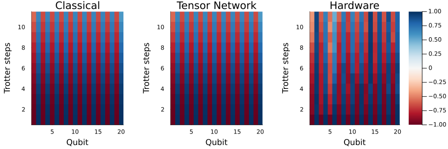
Mula sa mga bitstring sample na nakuha sa quantum hardware, kinukwenta natin ang magnetization kada site (ang mga single-qubit expectation value) sa pamamagitan ng pag-average ng sa lahat ng shot, kung saan ang ay ang nasukat na bit para sa qubit . Pagkatapos ay ipinaplano natin ang magnetization bilang heatmap sa mga qubit at Trotter step, na pinaghahambing ang tatlong method nang magkakatabi: eksaktong classical simulation, noiseless tensor network simulation, at pagpapatakbo sa hardware.
# Compute expectation values
# 0 -> 1, 1 -> -1
z_expval(samples, i) = mean((-1)^s[i] for s in samples)

magnetizations = [z_expval(all_samples[i], q) for i in 1:length(all_samples), q in 1:N]
11×20 Matrix{Float64}:
 -0.996094  0.998047  -0.990234  0.998047  …  1.0       -0.988281  0.994141
 -0.925781  0.980469  -0.878906  0.96875      0.970703  -0.976562  0.988281
 -0.916016  0.992188  -0.837891  0.957031     0.962891  -0.966797  0.953125
 -0.884766  0.970703  -0.824219  0.90625      0.908203  -0.939453  0.892578
 -0.835938  0.96875   -0.814453  0.884766     0.931641  -0.902344  0.908203
 -0.777344  0.958984  -0.78125   0.871094  …  0.935547  -0.876953  0.939453
 -0.732422  0.933594  -0.767578  0.8125       0.884766  -0.835938  0.890625
 -0.650391  0.916016  -0.771484  0.771484     0.853516  -0.773438  0.837891
 -0.537109  0.902344  -0.705078  0.742188     0.875     -0.662109  0.833984
 -0.472656  0.923828  -0.652344  0.728516     0.839844  -0.695312  0.808594
 -0.4375    0.923828  -0.613281  0.681641  …  0.890625  -0.658203  0.8125
Ipinapakita ng tatlong panel sa ibaba ang site magnetization na bilang function ng qubit index (x-axis) at Trotter step (y-axis). Sa at , ang kabuuang oras ng ebolusyon ay , na sapat na maikli kaya hindi pa nawawala ang paunang antiferromagnetic na pattern — lahat ng tatlong method ay nagpapakita ng malakas na magkakahalinhinang pattern. Malapit na nagkakasundo na ngayon ang mga resulta ng classical at tensor network, na nagpapatunay na maliit ang Trotter error sa laki ng step na ito. Sa pangkalahatan ay sinusundan ng mga resulta ng hardware ang dalawa pa, bagaman ang ilang qubit ay mas lumilihis sa mga simulation kaysa sa iba, na sumasalamin sa pagkakaiba-iba ng kalidad ng qubit sa buong backend. Lumalaki ang mga paglihis na ito sa mas huling Trotter step habang tumataas ang circuit depth.
# plot magnetization as a function of time
l = @layout [a{0.3w} b{0.3w} c{0.44w}]
plot(
    heatmap(classical_magnetizations, title="Classical", clims=(-1,1), color=:RdBu,
        xlabel="Qubit", ylabel="Trotter steps", colorbar=false),
    heatmap(tn_magnetizations, title="Tensor Network", clims=(-1,1), color=:RdBu,
        xlabel="Qubit", ylabel="Trotter steps", colorbar=false),
    heatmap(magnetizations, title="Hardware", clims=(-1,1), color=:RdBu,
        xlabel="Qubit", ylabel="Trotter steps", colorbar=true),
    layout=l, size=(900,300),
    bottom_margin=5mm, left_margin=5mm, right_margin=6mm
)
Halimbawa ng malaking hardware
Mga Hakbang 1–4 sa iisang workflow
Pinagsasama na natin ngayon ang lahat ng apat na hakbang sa itaas sa iisang workflow, sa laking hindi na maaabot ng eksaktong classical simulation. Sa halip na lutasin ang magnetization kada site, sinusubaybayan natin ang iisang scalar na sukat ng antiferromagnetic order, ang staggered magnetization:
Ang magkakahalinhinang sign sa summation ang nagpapakita ng signal. Para sa paunang Néel state na , bawat termino ay nag-aambag ng , kaya , samantalang ang simpleng average na ay zero para sa lahat ng . Habang ginugulo ng transverse field ang magkakahalinhinang pattern, bumababa ang papunta sa , kaya sinasabi sa atin ng staggered magnetization kung gaano karami sa paunang order ang nananatili habang nagaganap ang time evolution.
Ginagamit din natin ang halimbawang ito para makita kung paano nakakaapekto ang laki ng Trotter step sa katumpakan. Itinatakda natin ang kabuuang oras ng ebolusyon na at binabago ang bilang ng mga Trotter step na , kaya . Sa hardware, dalawang pinagmumulan ng error ang nagtutunggali: ang mas maliit na ay nagpapababa ng Trotter error, ngunit nangangailangan ng proporsyonal na mas maraming two-qubit gate, na nag-iipon ng mas maraming noise ng hardware.
# -------------------------Step 1-------------------------
# Map classical inputs to a quantum problem.
N_large = 100
g_large = named_grid((N_large,))
h_large = fill(1.0, N_large)       # transverse field on every site
J_large = fill(1.0, N_large - 1)   # nearest-neighbor ZZ couplings on the chain

T_total = 1.5                    # fixed total evolution time
r_list = [3, 6, 12]       # varying Trotter steps; δt = T_total/r
sweep = [(r, k) for r in r_list for k in 0:r]

qc_list_large = [make_trotter_circuit(h_large, J_large, N_large, T_total/r, k)
                 for (r, k) in sweep]

# -------------------------Step 2-------------------------
# Optimize the problem for quantum hardware execution.
tqc_list_large = [transpile(qc, target)[1] for qc in qc_list_large]
# Print the 2q gate count and depth of the deepest circuit at each δt",
for r in r_list
    i = findfirst(==((r, r)), sweep)   # the k = r circuit reaches the full T_total
    println("  δt = $(round(T_total/r, digits=4))  →  $(r+1) time points, ",
        "deepest circuit = $(r) Trotter steps, ",
        "2q count = $(two_qubit_count(tqc_list_large[i])), ",
        "2q depth = $(two_qubit_depth(tqc_list_large[i]))")
end

# -------------------------Step 3-------------------------
# Execute using Qiskit primitives.
shots_large = 4096

job_list_large = [run_sampler_job(service, backend, tqc, shots_large)
                  for tqc in tqc_list_large]
δt = 0.5  →  4 time points, deepest circuit = 3 Trotter steps, 2q count = 594, 2q depth = 206
  δt = 0.25  →  7 time points, deepest circuit = 6 Trotter steps, 2q count = 1188, 2q depth = 218
  δt = 0.125  →  13 time points, deepest circuit = 12 Trotter steps, 2q count = 2376, 2q depth = 242
24-element Vector{QiskitIBMRuntime.Job}:
 QiskitIBMRuntime.Job(Ptr{QiskitIBMRuntime.LibQiskitIBMRuntime.Job} @0x0000000104c1a750)
 QiskitIBMRuntime.Job(Ptr{QiskitIBMRuntime.LibQiskitIBMRuntime.Job} @0x0000000102e0a270)
 QiskitIBMRuntime.Job(Ptr{QiskitIBMRuntime.LibQiskitIBMRuntime.Job} @0x0000000104c21a50)
 QiskitIBMRuntime.Job(Ptr{QiskitIBMRuntime.LibQiskitIBMRuntime.Job} @0x0000000102e05120)
 QiskitIBMRuntime.Job(Ptr{QiskitIBMRuntime.LibQiskitIBMRuntime.Job} @0x0000000104c2a6e0)
 QiskitIBMRuntime.Job(Ptr{QiskitIBMRuntime.LibQiskitIBMRuntime.Job} @0x0000000102e0d140)
 QiskitIBMRuntime.Job(Ptr{QiskitIBMRuntime.LibQiskitIBMRuntime.Job} @0x0000000102e0b640)
 QiskitIBMRuntime.Job(Ptr{QiskitIBMRuntime.LibQiskitIBMRuntime.Job} @0x0000000104c1a200)
 QiskitIBMRuntime.Job(Ptr{QiskitIBMRuntime.LibQiskitIBMRuntime.Job} @0x00000004b312eb90)
 QiskitIBMRuntime.Job(Ptr{QiskitIBMRuntime.LibQiskitIBMRuntime.Job} @0x0000000104c22060)
 QiskitIBMRuntime.Job(Ptr{QiskitIBMRuntime.LibQiskitIBMRuntime.Job} @0x00000004b31ea4e0)
 QiskitIBMRuntime.Job(Ptr{QiskitIBMRuntime.LibQiskitIBMRuntime.Job} @0x0000000104c1ccf0)
 QiskitIBMRuntime.Job(Ptr{QiskitIBMRuntime.LibQiskitIBMRuntime.Job} @0x0000000104c2af50)
 QiskitIBMRuntime.Job(Ptr{QiskitIBMRuntime.LibQiskitIBMRuntime.Job} @0x00000004b312ffb0)
 QiskitIBMRuntime.Job(Ptr{QiskitIBMRuntime.LibQiskitIBMRuntime.Job} @0x00000004b0e89700)
 QiskitIBMRuntime.Job(Ptr{QiskitIBMRuntime.LibQiskitIBMRuntime.Job} @0x0000000102e15070)
 QiskitIBMRuntime.Job(Ptr{QiskitIBMRuntime.LibQiskitIBMRuntime.Job} @0x0000000102e10d40)
 QiskitIBMRuntime.Job(Ptr{QiskitIBMRuntime.LibQiskitIBMRuntime.Job} @0x00000004af5a5d10)
 QiskitIBMRuntime.Job(Ptr{QiskitIBMRuntime.LibQiskitIBMRuntime.Job} @0x0000000102e12500)
 QiskitIBMRuntime.Job(Ptr{QiskitIBMRuntime.LibQiskitIBMRuntime.Job} @0x0000000102e14870)
 QiskitIBMRuntime.Job(Ptr{QiskitIBMRuntime.LibQiskitIBMRuntime.Job} @0x0000000102e10730)
 QiskitIBMRuntime.Job(Ptr{QiskitIBMRuntime.LibQiskitIBMRuntime.Job} @0x00000004b237ca60)
 QiskitIBMRuntime.Job(Ptr{QiskitIBMRuntime.LibQiskitIBMRuntime.Job} @0x00000004b2c713a0)
 QiskitIBMRuntime.Job(Ptr{QiskitIBMRuntime.LibQiskitIBMRuntime.Job} @0x0000000102e13e90)
# Run this cell to check the job status
# Run the following cell for post-processing after all jobs complete
for (i, job) in enumerate(job_list_large)
    r, k = sweep[i]
    println("Job $i (δt=$(round(T_total/r, digits=4)), k=$k): ",
            get_job_status(job, service))
end
Job 1 (δt=0.5, k=0): Completed
Job 2 (δt=0.5, k=1): Completed
Job 3 (δt=0.5, k=2): Completed
Job 4 (δt=0.5, k=3): Completed
Job 5 (δt=0.25, k=0): Completed
Job 6 (δt=0.25, k=1): Completed
Job 7 (δt=0.25, k=2): Completed
Job 8 (δt=0.25, k=3): Completed
Job 9 (δt=0.25, k=4): Completed
Job 10 (δt=0.25, k=5): Completed
Job 11 (δt=0.25, k=6): Completed
Job 12 (δt=0.125, k=0): Completed
Job 13 (δt=0.125, k=1): Completed
Job 14 (δt=0.125, k=2): Completed
Job 15 (δt=0.125, k=3): Completed
Job 16 (δt=0.125, k=4): Completed
Job 17 (δt=0.125, k=5): Completed
Job 18 (δt=0.125, k=6): Completed
Job 19 (δt=0.125, k=7): Completed
Job 20 (δt=0.125, k=8): Completed
Job 21 (δt=0.125, k=9): Completed
Job 22 (δt=0.125, k=10): Completed
Job 23 (δt=0.125, k=11): Completed
Job 24 (δt=0.125, k=12): Completed
# -------------------------Step 4-------------------------
# Post-process and return the result in the desired classical format.
# Run this cell after all jobs are completed

# ⟨M_s⟩ = (1/N) Σ (-1)^i ⟨Z_i⟩, averaged over hardware shots
function staggered_magnetization(samples::AbstractVector{<:AbstractVector}, n::Int)
    s = 0.0
    for sample in samples
        s += sum((-1)^i * (1 - 2 * sample[i]) for i in 1:n) / n
    end
    return s / length(samples)
end

all_samples_large = [get_sampler_job_results(job, service) for job in job_list_large]
mags_hardware = [staggered_magnetization(s, N_large) for s in all_samples_large]
24-element Vector{Float64}:
 0.9880371093750097
 0.697231445312484
 0.44886718750000276
 0.29333496093750067
 0.9882324218750095
 0.8109619140625324
 0.6457958984374791
 0.4808593749999992
 0.36695312500000055
 0.2963671875000012
 0.23831542968750055
 0.9884472656250093
 0.8566455078125492
 0.7951171875000282
 0.7050732421874865
 0.610673828124981
 0.529980468749995
 0.4656054687500018
 0.4149316406250024
 0.3799462890625011
 0.35178710937500185
 0.3185888671875003
 0.31287597656250016
 0.29621093750000077
Sa , hindi maaabot ang eksaktong solusyon mula sa ODE solver na ginamit sa itaas, dahil ang state vector pa lang ay mangangailangan ng amplitude. Sa halip, gumagamit tayo ng noiseless tensor network simulation ng parehong 1D chain na may mas pinong Trotter step (, ) bilang reference, kung saan bale-wala ang Trotter error kumpara sa anumang na pinapatakbo natin sa hardware. Tinatayang halaga rin ang reference na ito: ang pangunahing error nito ngayon ay ang bond-dimension truncation na tinalakay sa itaas, na iniuulat bilang truncation fidelity para sa bawat run.
apply_kwargs = (; maxdim=64, cutoff=1e-10, normalize_tensors=true)

# Calculate the staggered magnetization given a tensor network state
staggered_magnetization(ψ_bpc::BeliefPropagationCache, n::Int) =
    sum((-1)^q * m for (q, m) in enumerate(z_expvals_from_tn_state(ψ_bpc, n))) / n

# Evolve a TN state and record the staggered magnetization at each step.
function compute_staggered_magnetization_tn(δt::Real, nsteps::Int; record_every::Int = 1)
    init_gates = neel_state_gates(N_large)
    step_gates = trotter_step_gates(h_large, J_large, N_large, δt)

    ψ_bpc, fid = apply_gates_to_tn_state(init_gates, tn_initial_state(g_large); apply_kwargs)
    times = [0.0]
    mags = [staggered_magnetization(ψ_bpc, N_large)]
    for k in 1:nsteps
        ψ_bpc, fid_step = apply_gates_to_tn_state(step_gates, ψ_bpc; apply_kwargs)
        fid *= fid_step
        if k % record_every == 0
            push!(times, k * δt)
            push!(mags, staggered_magnetization(ψ_bpc, N_large))
        end
    end
    println("  δt=$(round(δt, digits=5)), $(nsteps) steps: truncation fidelity ≈ $(round(fid, digits=5))")
    (times, mags)
end

# If the fidelity drifts from 1, raise `maxdim` in `apply_kwargs`.
# Under current setting, the tensor network simulation takes ~ 3 minutes on a laptop.
println("Tensor-network reference:")
r_ref = 96
times_ref, mags_ref = compute_staggered_magnetization_tn(T_total / r_ref, r_ref; record_every = r_ref ÷ 12)
Tensor-network reference:
  δt=0.01562, 96 steps: truncation fidelity ≈ 1.0
([0.0, 0.125, 0.25, 0.375, 0.5, 0.625, 0.75, 0.875, 1.0, 1.125, 1.25, 1.375, 1.5], Float32[1.0, 0.9695576, 0.8870231, 0.77430177, 0.6560442, 0.5499543, 0.46285573, 0.39298016, 0.33518773, 0.28527063, 0.24147007, 0.20369667, 0.17206171])
Ipinapakita ng plot sa ibaba ang staggered magnetization sa paglipas ng oras para sa tatlong laki ng Trotter step, kumpara sa noiseless tensor network reference (putol-putol na itim).
plt = plot(xlabel = "Time", ylabel = "Staggered magnetization",
    title = "N = $(N_large) on $(backend.name), T = $(T_total)",
    legend = :topright, ylims = (-0.05, 1.05), size = (820, 480),
    bottom_margin = 5mm, left_margin = 5mm)

# Plot tensor network reference
plot!(plt, times_ref, mags_ref, lw = 2, ls = :dash, color = :black,
      label = "tensor network, δt → 0")

# Plot hardware result per Trotter step size
for (r, stop) in zip(r_list, cumsum(r_list .+ 1))
    plot!(plt, range(0, T_total, length = r + 1), mags_hardware[(stop - r):stop],
          marker = :circle, markersize = 4, lw = 2,
          label = "hardware, δt = $(round(T_total / r, digits = 4))")
end
plt
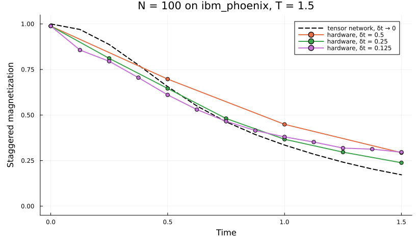
Sa kabuuan, ang pinakamagaspang na Trotter step na (orange na tuldok) ang may pinakamalaking paglihis mula sa tensor network reference, na marahil ay may malaking ambag mula sa Trotter error. Sa mas pinong step na (berdeng tuldok), mas malapit na nagkakasundo ang mga resulta ng hardware sa reference. Sa pinakapinong step na (lilang tuldok), pinakamaliit ang Trotter error, ngunit mas malala ang pagkakasundo kaysa sa . Kapag kalahati ang laki ng step, bawat time point ay nangangailangan ng dalawang beses na mas maraming two-qubit gate, at ang karagdagang noise ay lampas sa pagbaba ng Trotter error. Kaya ang pagpili ng para sa isang Trotterized circuit sa hardware ay isang trade-off sa pagitan ng Trotter error at ng noise na naiipon mula sa karagdagang mga gate.
Mga susunod na hakbang
Maaaring interesado ka sa mga sumusunod na materyal: