Hanapin ang Maximum Independent Set gamit ang Aqarios Constrained Quantum Optimizer

Tandaan

Ang Qiskit Functions ay isang experimental feature na available lamang sa IBM Quantum® Premium Plan, Flex Plan, at On-Prem (sa pamamagitan ng IBM Quantum Platform API) Plan users. Ito ay nasa preview release status at maaaring magbago.

Tinatayang paggamit: 30 segundo sa isang Heron r2 processor. (TANDAAN: Isa lamang itong pagtatantya. Maaaring mag-iba ang iyong runtime.)

Kaligiran

Ipinapakita ng tutorial na ito kung paano hanapin ang maximum independent set ng isang graph gamit ang Aqarios Constrained Quantum Optimizer [1], isang constrained combinatorial optimization problem. Ang isang instance mula sa QOBLIB [2] benchmark library ay binubuo bilang binary linear program at ipinapasa sa Optimizer Application Function. Ang optimizer ang bahalang humawak sa lahat ng reformulation, circuit synthesis, transpilation, at iterative warm starting sa loob mismo (tingnan ang [3] para sa detalye).

Saklaw ng tutorial ang mga sumusunod na hakbang:

1. I-define ang problema bilang linear program gamit ang OptimizationProblem mula sa qiskit-addon-opt-mapper

2. Patakbuhin ang quantum optimization gamit ang Aqarios Constrained Quantum Optimizer

3. Kunin at i-visualize ang mga resulta

Ang Maximum Independent Set problem

Ang Maximum Independent Set (MIS) problem ay isang pangunahing hamon sa combinatorial optimization. Formally, sa ibinigay na graph $G(V, E)$, ang layunin ay hanapin ang pinakamalaking subset ng vertices $V_I \subset V$ kung saan walang dalawang vertex sa $V_I$ na konektado ng isang edge, tulad ng $\nexists (u, v) \in E : v \in V_I \wedge u \in V_I$. Bawat vertex ay binibigyan ng binary decision variable $x_i \in \{0, 1\}$, at isang constraint $x_u + x_v \leq 1$ ay ipinapasok para sa bawat edge, para matiyak na hindi hihigit sa isang endpoint ng bawat edge ang mapipili. Sa gayon, maaaring sabihin ang problema bilang sumusunod na maximization problem:

$$\max_{x_i} \sum_{i \in V} x_i \qquad\text{(hanapin ang pinakamalaking set)}\\ \text{s.t.} \quad x_u + x_v \leq 1 \quad \forall (u, v) \in E.$$

Malawak ang praktikal na aplikasyon ng MIS. Sa wireless network planning, ang independent set ay tumutugma sa isang grupo ng mga transmitter na maaaring lahat mag-broadcast nang sabay-sabay nang walang mutual interference. Sa scheduling, minomodelo nito ang pinakamalaking koleksyon ng mga task na maaaring maisagawa nang sabay-sabay na isinasaalang-alang ang pairwise resource conflicts. Sa computational biology, hinuhuli nito ang mga set ng mutually non-interacting proteins sa isang network.

Sa kabila ng intuitive na formulation nito, ang MIS ay NP-hard, at kahit para sa mga graph na may ilang daang nodes, nagiging mahirap lutasin nang eksakto o heuristically ang ilang partikular na instance [2]. Ang problema ay nagbibigay din ng sparse constraint structures na angkop para sa hardware implementations ng quantum optimization, kaya't ito ay naging kaakit-akit na benchmark para sa near-term quantum devices.

Aqarios Constrained Quantum Optimizer

Ang standard approach para i-embed ang isang constrained binary problem sa quantum optimization ay nagbabago sa model tungo sa unconstrained format sa pamamagitan ng pagdagdag ng penalty terms: ang bawat nilabag na constraint $x_u + x_v \leq 1$ ay nag-aambag ng $2 x_u x_v$ sa minimization objective $-\sum_i x_i$. Ito ay awtomatikong hinahawakan ng Constrained Quantum Optimizer Qiskit Function.

Higit pa sa standard transformation na ito, tinutukoy ng optimizer ang mga cliques sa constraint graph. Ang clique ay isang set ng mga node $V_C$ kung saan ang bawat pares ng node ay may shared na edge. Bunga nito, ang $\binom{|V_C|}{2}$ pairwise constraints $x_u + x_v \leq 1 \;\forall (u,v) \in E_C$ ay maaaring palitan ng iisa at mas mahigpit na constraint $\sum_{i \in V_C} x_i \leq 1$. Ang pagpapakilala ng slack variable $y$ ay nagpapalit nito sa equality $\sum_i x_i + y = 1$, na kumukuha ng anyo ng one-hot constraint na maaaring direktang i-enforce sa QAOA gamit ang XY-mixers [3]. Binabawasan nito ang search space at iniiwasan ang pangangailangan ng penalty terms para sa mga constraint na iyon, na nagpapabuti sa kalidad ng solusyon.

Bukod dito, ang mga variable na konektado lamang sa iisang neighbor ay tinatawag na pendant nodes at ito ay deterministikong ini-fix ng algorithm bago ang quantum execution, na lalong nagpapababa sa effective problem size.

Gumagamit ang Constrained Quantum Optimizer ng iterative warm-starting approach na compatible sa XY-mixers [1], na paunti-unting nagpapaliit sa search space sa pamamagitan ng pag-bias sa quantum state distribution patungo sa mga promising na solution regions sa bawat iteration. Ito ay nagbibigay-daan sa paggamit ng fixed-angle QAOA parameters, na inaalis ang pangangailangan para sa variational parameter training. Ang kabuuang quantum resource requirements ay dikta lamang ng bilang ng warm-start iterations, na nangangahulugang diretso lang i-control ang quantum cost.

Mga Kailangan

Bago simulan ang tutorial na ito, siguraduhing na-install mo na ang mga sumusunod na requirements:

• Qiskit Runtime (pip install qiskit-ibm-runtime)

• Qiskit Functions Catalog IBM Client (pip install qiskit-ibm-catalog)

• Qiskit Addon Optimization Mapper (pip install qiskit-addon-opt-mapper)

• Numpy (pip install numpy)

• Matplotlib (pip install matplotlib)

• NetworkX (pip install networkx)

Opsyonal, para sa Appendix kailangan mong i-install

• Luna Model (pip install luna-model)

Pag-setup

I-import ang lahat ng kinakailangang dependencies.

# Added by doQumentation — installs the packages this notebook needs if they are missing
import importlib.util

_needed = {"luna_model": "luna-model", "networkx": "networkx", "numpy": "numpy", "qiskit_addon_opt_mapper": "qiskit-addon-opt-mapper", "qiskit_ibm_catalog": "qiskit-ibm-catalog"}
_missing = [pip for module, pip in _needed.items()
            if importlib.util.find_spec(module) is None]
# One at a time, so a package that fails to install does not block the others
for _pip in _missing:
    %pip install -q {_pip}
if not _missing:
    print("\u2713 All required packages are installed")

import networkx as nx
import urllib.request

from qiskit_ibm_catalog import QiskitFunctionsCatalog

from qiskit_addon_opt_mapper import OptimizationProblem
from qiskit_addon_opt_mapper.applications import IndependentSet
from qiskit_addon_opt_mapper.translators import to_docplex_mp

Una, mag-authenticate gamit ang iyong IBM Quantum API key. Pagkatapos, piliin ang Qiskit Function gaya ng sumusunod. (Ipinapalagay ng code na ito na na-save mo na ang iyong account sa iyong local environment.)

catalog = QiskitFunctionsCatalog(channel="ibm_quantum_platform")

# Verify that you have access to the function
catalog.list()

[QiskitFunction(aqarios/constrained-quantum-optimizer)]

# Load the function
optimizer = catalog.load("aqarios/constrained-quantum-optimizer")

# Check the list of backends you have access to
catalog.backends()

[<IBMBackend('ibm_pittsburgh')>,
 <IBMBackend('ibm_boston')>,
 <IBMBackend('ibm_phoenix')>,
 <IBMBackend('ibm_fez')>,
 <IBMBackend('ibm_miami')>,
 <IBMBackend('ibm_marrakesh')>,
 <IBMBackend('ibm_kingston')>]

# Select the backend you want to use
backend = catalog.backend("ibm_pittsburgh")

Hakbang 1: I-map ang classical inputs sa quantum problem

Ang problema ay binubuo bilang isang LP-file, isang karaniwang format para sa optimization problems na siyang ginagamit bilang input sa Aqarios Constrained Quantum Optimizer. Bukod sa LP-files, sinusuportahan din ng function ang MPS-files at native Luna Model representations. Ginagawa ang LP-file sa pamamagitan ng mga sumusunod na hakbang:

1. Kunin ang isang graph instance mula sa QOBLIB [2]

2. I-model ang optimization problem

3. Buuin ang LP-file

I-load ang problem instance graph

Ang mga graph ay tinukoy sa DIMACS .gph format, isang line-based na format kung saan ang mga linyang nagsisimula sa e ay naglalarawan ng edges, ang mga linyang nagsisimula sa p ay naglalarawan ng problem header, at ang mga linyang nagsisimula sa c ay mga comment:

c some-comment
p edge 3 2
e 1 2
e 2 3
...

Ang .gph file ay maaaring i-download mula sa QOBLIB repository gamit ang sumusunod na function, na nagpa-parse din nito tungo sa isang NetworkX graph. Pansinin na ang DIMACS format ay gumagamit ng 1-based node labeling, na kino-convert dito tungo sa 0-based indexing.

URL_BASE = "https://raw.githubusercontent.com/ZIB-AOPT/QOBLIB/refs/heads/main/07-independentset/instances/"

def fetch_qoblib_graph(name: str) -> nx.Graph:
    """Fetch and parse the QOBLIB graph file."""
    # Download the .gph file
    file, _ = urllib.request.urlretrieve(URL_BASE + f"{name}.gph")
    with open(file) as f:
        # Read the file contents
        lines = f.readlines()

    # Skip comments
    lines = [line for line in lines if not line.startswith("c")]

    # Read graph definition
    _, _, num_nodes, num_edges = lines[0].split()
    print(f"Loading graph with {num_nodes} nodes and {num_edges} edges.")

    # Parse edge information
    # The .gph format starts node labeling with 1; we need 0 here, so we subtract one.
    split_edges = (line.split() for line in lines[1:])
    edges = [(int(u) - 1, int(v) - 1) for _, u, v in split_edges]

    return nx.Graph(edges)

graph_name = "es60fst02"
graph = fetch_qoblib_graph(graph_name)

Loading graph with 186 nodes and 280 edges.

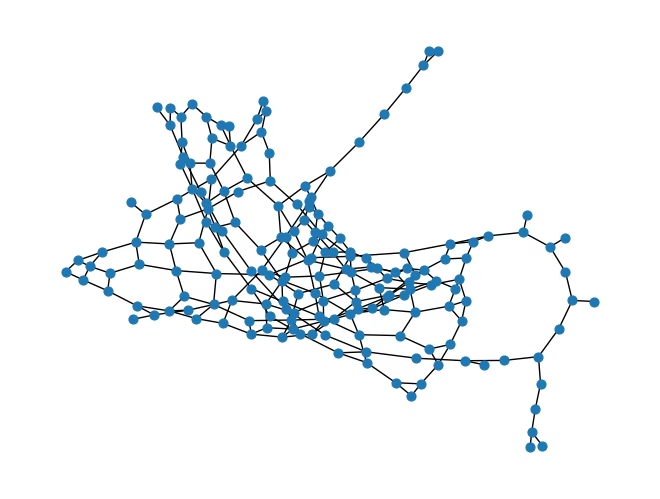
Ginagamit ng halimbawang ito ang es60fst02 instance mula sa QOBLIB, isang graph na may 186 nodes at 280 edges. Salamat sa preprocessing steps na ginagamit ng Constrained Quantum Optimizer, ang instance na ito ay malulutas sa 156-qubit na Heron devices. Ang graph ay maaaring i-visualize gamit ang matplotlib:

# Keep layout for later reuse
layout = nx.spring_layout(graph, seed=1)
nx.draw(graph, layout, node_size=40)

Buuin ang optimization problem

Ang Maximum Independent Set problem ay maaaring direktang buuin gamit ang OptimizationProblem. Ang bawat graph node ay nagiging binary decision variable, at ang bawat edge ay nagpapakilala ng constraint na sinisiguro na hindi hihigit sa isa sa mga endpoint nito ang mapipili:

# Create an OptimizationProblem instance
mis_problem = OptimizationProblem("MIS")

# Add a binary variable for each node
x = mis_problem.binary_var_list(graph.number_of_nodes())

# Maximize the sum of all node variables
mis_problem.maximize(linear={xi.name: 1 for xi in x})

# Add '<= 1' constraints for each edge
for u, v in graph.edges:
    mis_problem.linear_constraint({x[u].name: 1, x[v].name: 1}, "<=", 1)

Isang shortcut

Ang qiskit-addon-opt-mapper package ay nagbibigay ng pre-implemented na application class para sa Maximum Independent Set problem, na nagpapadali sa formulation sa itaas tungo sa iisang tawag:

mis = IndependentSet(graph)
mis_problem = mis.to_optimization_problem()

I-translate ang problema tungo sa LP-file

Ang OptimizationProblem mismo ay hindi sumusuporta sa LP-file exports, ngunit ito ay interoperable sa DOcplex, na sumusuporta nito. Dalawang linya lamang ang kailangan para makabuo ng LP-file contents:

mp_model = to_docplex_mp(mis_problem)
lp_str = mp_model.export_as_lp_string()

print("\n".join(lp_str.split("\n")[:60]))
print("...")

\ This file has been generated by DOcplex
\ ENCODING=ISO-8859-1
\Problem name: Independent set

Maximize
 obj: x_0 + x_1 + x_2 + x_3 + x_4 + x_5 + x_6 + x_7 + x_8 + x_9 + x_10 + x_11
      + x_12 + x_13 + x_14 + x_15 + x_16 + x_17 + x_18 + x_19 + x_20 + x_21
      + x_22 + x_23 + x_24 + x_25 + x_26 + x_27 + x_28 + x_29 + x_30 + x_31
      + x_32 + x_33 + x_34 + x_35 + x_36 + x_37 + x_38 + x_39 + x_40 + x_41
      + x_42 + x_43 + x_44 + x_45 + x_46 + x_47 + x_48 + x_49 + x_50 + x_51
      + x_52 + x_53 + x_54 + x_55 + x_56 + x_57 + x_58 + x_59 + x_60 + x_61
      + x_62 + x_63 + x_64 + x_65 + x_66 + x_67 + x_68 + x_69 + x_70 + x_71
      + x_72 + x_73 + x_74 + x_75 + x_76 + x_77 + x_78 + x_79 + x_80 + x_81
      + x_82 + x_83 + x_84 + x_85 + x_86 + x_87 + x_88 + x_89 + x_90 + x_91
      + x_92 + x_93 + x_94 + x_95 + x_96 + x_97 + x_98 + x_99 + x_100 + x_101
      + x_102 + x_103 + x_104 + x_105 + x_106 + x_107 + x_108 + x_109 + x_110
      + x_111 + x_112 + x_113 + x_114 + x_115 + x_116 + x_117 + x_118 + x_119
      + x_120 + x_121 + x_122 + x_123 + x_124 + x_125 + x_126 + x_127 + x_128
      + x_129 + x_130 + x_131 + x_132 + x_133 + x_134 + x_135 + x_136 + x_137
      + x_138 + x_139 + x_140 + x_141 + x_142 + x_143 + x_144 + x_145 + x_146
      + x_147 + x_148 + x_149 + x_150 + x_151 + x_152 + x_153 + x_154 + x_155
      + x_156 + x_157 + x_158 + x_159 + x_160 + x_161 + x_162 + x_163 + x_164
      + x_165 + x_166 + x_167 + x_168 + x_169 + x_170 + x_171 + x_172 + x_173
      + x_174 + x_175 + x_176 + x_177 + x_178 + x_179 + x_180 + x_181 + x_182
      + x_183 + x_184 + x_185
Subject To
 c0: x_60 + x_61 <= 1
 c1: x_14 + x_60 <= 1
 c2: x_7 + x_60 <= 1
 c3: x_7 + x_61 <= 1
 c4: x_61 + x_62 <= 1
 c5: x_61 + x_64 <= 1
 c6: x_14 + x_62 <= 1
 c7: x_62 + x_65 <= 1
 c8: x_23 + x_63 <= 1
 c9: x_53 + x_63 <= 1
 c10: x_39 + x_63 <= 1
 c11: x_7 + x_68 <= 1
 c12: x_18 + x_68 <= 1
 c13: x_68 + x_69 <= 1
 c14: x_68 + x_72 <= 1
 c15: x_64 + x_65 <= 1
 c16: x_64 + x_69 <= 1
 c17: x_65 + x_66 <= 1
 c18: x_51 + x_53 <= 1
 c19: x_69 + x_73 <= 1
 c20: x_66 + x_67 <= 1
 c21: x_42 + x_66 <= 1
 c22: x_67 + x_75 <= 1
 c23: x_43 + x_67 <= 1
 c24: x_42 + x_75 <= 1
 c25: x_75 + x_83 <= 1
 c26: x_12 + x_51 <= 1
 c27: x_18 + x_70 <= 1
 c28: x_18 + x_26 <= 1
 c29: x_70 + x_71 <= 1
 c30: x_70 + x_76 <= 1
 c31: x_71 + x_72 <= 1
 c32: x_72 + x_73 <= 1
 c33: x_72 + x_78 <= 1
...

Ang format na ito ay native sa Constrained Quantum Optimizer.

Hakbang 2: I-optimize ang problema para sa quantum hardware execution

Ang lahat ng circuit synthesis, optimization, at transpilation ay hinahawakan ng function nang natively. Tingnan ang inputs section sa API reference para sa mga argumento na gagamitin sa pagtawag ng function.

Para i-fine-tune ang behavior ng algorithm, tingnan ang Options list sa API reference. Kung gusto mong maging reproducible ang circuit mapping sa bawat takbo, i-fix ang opsyong seed_transpiler.

Para sa karagdagang impormasyon, tingnan ang Aqarios Constrained Quantum Optimizer guide at API reference.

Hakbang 3: Isagawa gamit ang Qiskit primitives

Ang LP-file ay maaari nang isumite sa optimizer:

job = optimizer.run(problem=lp_str, backend_name=backend.name)

print(f"Job ID: {job.job_id}")

Job ID: 87ec08b9-6275-40fa-be94-340a0a916bf1

Sa loob mismo, dumadaan ang algorithm sa mga sumusunod na stages:

1. Preprocessing:

   • Bawasan ang mga fixable variables

   • Hanapin ang mga clique

   • Tukuyin ang mga uri ng constraint

   • Suriin ang mga penalty factors para sa penalty terms

   • I-apply ang constraint transformations

   • Buuin ang circuit gamit ang constraint-enforcing methods

   • Approximation ng problema at transpilation

2. Parallel chains ng iterative loops:

   • Mag-sample mula sa circuit gamit ang fixed parameters

   • I-apply ang postprocessing

   • Suriin at itakda ang bagong warm-starting probabilities

3. Postprocessing:

   • Hanapin ang mga pinakamahusay na sample at suriin ang feasibility patungkol sa input problem

Bantayan ang progress

Tingnan ang mga sumusunod na section sa Get started with Qiskit Functions page para bantayan ang progress ng iyong job:

• Suriin ang status ng job

• Kunin ang mga resulta

# Monitor the job status
job.status()

'QUEUED'

Hakbang 4: I-post-process at ibalik ang mga resulta sa gustong classical format

Ang result output ay isang dictionary, na ang mga field nito ay inilalarawan sa Outputs section ng API reference.

Kapag ang solutions list ay may higit sa isang entry, ibig sabihin ay maraming degenerate optima ang natagpuan. Ang unang solusyon lamang ang isinasaalang-alang dito, na tinutukoy sa pamamagitan ng pangalan ng variable. Available din ang parehong mga solusyon bilang mga bitstring sa solution_bitstrings, kung saan ibinibigay ng metadata.solver_info.variable_mapping ang posisyon ng karakter ng bawat variable.

# Retrieve the job result
result = job.result()

# Retrieve the first solution from the result
solution = result["solutions"][0]

print(f"The found maximum independent set of {graph_name} contains:", end=" ")
print(
    f"{int(result['objective_value'])} nodes and is {'feasible' if result['feasible'] else 'infeasible'}."
)
print("{" + " ".join(k[2:] for k, v in solution.items() if v == 1) + "}")

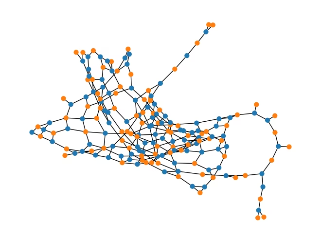
The found maximum independent set of es60fst02 contains: 88 nodes and is feasible.
{100 103 107 109 111 113 115 118 121 123 124 127 129 130 132 133 138 142 144 148 149 155 156 16 161 162 165 167 169 170 175 28 31 33 35 36 47 50 58 59 60 62 64 66 68 71 73 75 78 79 84 85 87 90 91 93 94 95 39 5 27 23 43 15 22 9 4 56 32 30 53 26 17 54 1 37 41 49 34 11 139 153 12 3 6 57 20 44}

Visualisasyon

Ang natukoy na independent set ay maaaring i-visualize sa pamamagitan ng pag-highlight sa mga napiling node sa graph:

# Color all selected nodes in orange
node_map = {
    int(k.split("_")[1]): "tab:orange" if v else "tab:blue"
    for k, v in solution.items()
}
node_colors = [node_map[k] for k in graph.nodes]

# Draw with the same layout used before
nx.draw(graph, layout, node_size=40, node_color=node_colors)

Appendix: Problem statement gamit ang Luna Model

Bukod sa qiskit-addon-opt-mapper approach na ipinakita sa itaas, tinatanggap din ng Qiskit Function ang mga model na ginawa gamit ang Luna Model [4], ang modeling SDK ng Aqarios. Matapos i-install ang luna-model PyPI package, i-import ito gaya ng sumusunod:

Setup:

from luna_model import Model, Sense
import numpy as np

Ang model ay binubuo mula sa graph sa parehong paraan tulad ng qiskit-addon-opt-mapper: Buuin ang model:

edges = np.array(graph.edges)

# Create the optimization model with a name
model = Model(name=f"MIS-{graph_name}", sense=Sense.MAX)
# Add binary variables
x = model.add_variables("x", graph.number_of_nodes())
# Set the objective
model.objective = x.sum()

# Use numpy like batch generation of constraints
model.add_constraints(x[edges].sum(axis=1) <= 1)

input_str = model.encode_b64()

# optimizer.run(problem=input_str, backend_name="ibm_fez")

Mga Susunod na Hakbang

Mga Rekomendasyon

• Sumangguni sa Aqarios Constrained Quantum Optimizer guide para sa detalyadong walkthrough ng lahat ng function features.
• Galugarin ang API reference para sa kumpletong listahan ng input parameters at output fields.
• Mag-eksperimento sa mga algorithm options (reps, num_parallel, shots, postprocessing_level) sa sarili mong constrained binary optimization problem para masuri ang epekto nito sa kalidad ng solusyon at runtime.

Mga Sanggunian

1. IBM Quantum, Aqarios Constrained Quantum Optimizer Guide

2. Koch et al. (2026), The Quantum Optimization Benchmarking Library 10.1038/s43588-026-00991-1

3. Bucher et al. (2026), Constrained Quantum Optimization via Iterative Warm-Start XY-Mixers 10.1088/1367-2630/ae8ea2

4. Aqarios GmbH, Luna Model Docs