Pagsisimula ng ergodicity sa iba't ibang scale
Tinatalakay ng notebook na ito kung paano patakbuhin at i-analyze ang mga experiment sa Onset of Ergodicity Across Scales on a Digital Quantum Processor [arXiv:2603.12236]: mula sa model hanggang sa mga Circuit, mula sa mga bitstring hanggang sa mga entropy, mula sa maingay na data hanggang sa mga na-mitigate na resulta, at mula sa 16-qubit na simulation hanggang sa 64-qubit na run sa isang IBM Quantum® Nighthawk processor. Narito ang lahat ng code, at ang bawat function ay dine-define kung saan ito unang kailangan.
| Oras | Seksyon |
|---|---|
| 0–1 min | Setup |
| 1–6 min | 1. Mula sa model hanggang sa Circuit |
| 6–12 min | 2. Ano ang susukatin at paano ito tantiyahin |
| 12–19 min | 3. Ang noise, at paano ito pawalang-bisa |
| 19–24 min | 4. Patakbuhin sa malaking scale |
| 24–33 min | 5. Ang data ng hardware |
| 33–35 min | Pangwakas |
Sumabay. Patakbuhin ang mga cell mula itaas hanggang ibaba. Hindi kailangan ng IBM Quantum account; naka-off ang mga cell na nagsa-submit ng mga hardware job, at sinusuri ng seksyon 5 ang isang naka-save na hardware run, na dina-download ng setup cell sa data/. Minarkahan ng Question ang mga tanong para sa talakayan; subukang sagutin bago mo buksan ang sagot.
Pag-set up
Nangangailangan ng Python 3.12 o mas bago at ng mga sumusunod na package:
-
Qiskit SDK v2.5 o mas bago, na may suporta sa visualization
-
Qiskit Runtime v0.49 o mas bago (
pip install qiskit-ibm-runtime) -
Qiskit Aer v0.17 o mas bago (
pip install qiskit-aer) -
Samplomatic v0.21 o mas bago (
pip install samplomatic) -
NumPy at Matplotlib
Dina-download din ng setup cell ang naka-save na hardware run at mga MPS reference (mga 9 MB) sa data/, maliban kung nandoon na ang mga ito.
# Added by doQumentation — installs the packages this notebook needs if they are missing
import importlib.util

_needed = {"matplotlib": "matplotlib", "numpy": "numpy", "qiskit": "qiskit", "qiskit_aer": "qiskit-aer", "qiskit_ibm_runtime": "qiskit-ibm-runtime", "samplomatic": "samplomatic"}
_missing = [pip for module, pip in _needed.items()
            if importlib.util.find_spec(module) is None]
# One at a time, so a package that fails to install does not block the others
for _pip in _missing:
    %pip install -q {_pip}
if not _missing:
    print("\u2713 All required packages are installed")
from math import comb
from pathlib import Path
from urllib.request import urlretrieve

import matplotlib.pyplot as plt
import numpy as np
from qiskit import ClassicalRegister, QuantumCircuit, QuantumRegister
from qiskit.primitives import StatevectorSampler
from qiskit.quantum_info import (
    PauliLindbladMap,
    QubitSparsePauli,
    Statevector,
)
from qiskit.transpiler import generate_preset_pass_manager
from qiskit_aer import AerSimulator
from qiskit_aer.noise import NoiseModel, ReadoutError, depolarizing_error
from qiskit_aer.primitives import SamplerV2 as AerSampler

RUN_ON_HARDWARE = (
    False  # True submits the 8x8 jobs in section 4 (needs Nighthawk access)
)
COMPUTE_MPS_REFERENCES = False  # True recomputes the MPS references in section 5 (about 18 minutes)

# Download the saved hardware run and MPS references, unless they are already in data/
data_url = "https://raw.githubusercontent.com/Qiskit/documentation/main/datasets/tutorials/onset-of-ergodicity"
Path("data").mkdir(exist_ok=True)
for name in ("hardware_run.npz", "mps_references_all.npz"):
    if not Path("data", name).exists():
        urlretrieve(f"{data_url}/{name}", Path("data", name))
1. Mula sa model hanggang sa Circuit
Ang two-qubit Gate
Ang bawat bond ng lattice ay nakakakuha ng parehong two-qubit Gate, na binubuo ng Heisenberg entangler na sinusundan ng mga random na field:
na may na iginuhit nang uniform mula sa para sa bawat Gate.
Question. Paano mo hahatiin ang sa mga Gate na kayang patakbuhin ng hardware?
Sagot
Ang mga field ay madali. Ang ay isang single-qubit rotation na sa bawat Qubit.
Ang entangler ang mahirap na bahagi. Nagko-commute ang , at , kaya nahahati ito sa tatlong rotation, , at . Bawat isa ay nangangailangan ng dalawang CNOT, na nagiging anim na CNOT bawat Gate.
May mas magandang paraan. Ang anumang two-qubit Gate ay mabubuo mula sa hindi hihigit sa tatlong CNOT at mga single-qubit rotation. Nagsisimula ang optimal na Circuit sa anyong , at ang entangler na ito ay may ganoong anyo na kapag . Kaya direkta itong napupunta sa tatlong CNOT, at linear sa ang mga single-qubit angle. Ganito binubuo ng experiment code ang Gate.
Sa hardware, nagdaragdag ng noise ang bawat two-qubit Gate, kaya mahalaga ang paghahati sa kalahati ng bilang ng CNOT.
def xxyyzz_gate(circuit, coupling, i, j):
    # exp(iJ(XX + YY + ZZ)) with three CNOTs; only the rotation angles depend on J
    circuit.rz(-np.pi / 2, j)
    circuit.cx(j, i)
    circuit.rz(np.pi / 2 - 2 * coupling, i)
    circuit.ry(2 * coupling - np.pi / 2, j)
    circuit.cx(i, j)
    circuit.ry(np.pi / 2 - 2 * coupling, j)
    circuit.cx(j, i)
    circuit.rz(np.pi / 2, i)

def heisenberg_gate(circuit, coupling, i, j, h_i, h_j):
    # The entangler first, then the random fields exp(i h Z)
    xxyyzz_gate(circuit, coupling, i, j)
    circuit.rz(-2 * h_i, i)
    circuit.rz(-2 * h_j, j)

h_i, h_j = 0.3, -0.7
gate = QuantumCircuit(2)
heisenberg_gate(gate, 0.05 * np.pi, 0, 1, h_i, h_j)
gate.draw("mpl")

Ang brickwork at ang Floquet cycle
Pinupuno ng mga Gate ang square lattice sa apat na sublayer ng mga hindi nagpapatong na bond, isang brickwork: mga pahalang na bond na nagsisimula sa mga even na column, pagkatapos mga odd na column, pagkatapos mga patayong bond na nagsisimula sa mga even na row, pagkatapos mga odd na row. Ang Qubit ay nasa site .
def brickwork_layers(num_cols, num_rows):
    # Bonds of the square lattice, in the four sublayers of the brickwork
    def qubit(x, y):
        return y * num_cols + x

    layers = []
    for p in (0, 1):  # horizontal bonds starting on even, then odd, columns
        layers.append(
            [
                (qubit(x, y), qubit(x + 1, y))
                for y in range(num_rows)
                for x in range(p, num_cols - 1, 2)
            ]
        )
    for p in (0, 1):  # vertical bonds starting on even, then odd, rows
        layers.append(
            [
                (qubit(x, y), qubit(x, y + 1))
                for y in range(p, num_rows - 1, 2)
                for x in range(num_cols)
            ]
        )
    return layers

brickwork_layers(4, 4)
[[(0, 1), (2, 3), (4, 5), (6, 7), (8, 9), (10, 11), (12, 13), (14, 15)],
 [(1, 2), (5, 6), (9, 10), (13, 14)],
 [(0, 4), (1, 5), (2, 6), (3, 7), (8, 12), (9, 13), (10, 14), (11, 15)],
 [(4, 8), (5, 9), (6, 10), (7, 11)]]
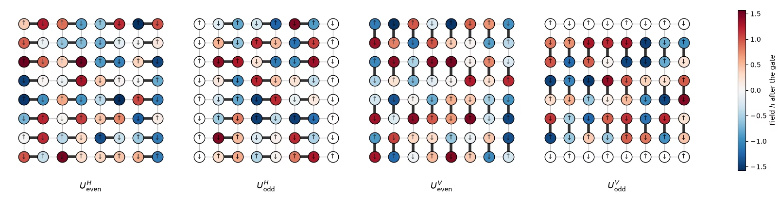
Ang apat na sublayer ay bumubuo ng isang Floquet cycle. Inuulit ang cycle nang beses gamit ang parehong mga field, kaya random sa espasyo at periodic sa oras ang dynamics. Nagsisimula ang Circuit sa Néel state, at ang ay kalahati ng haba ng gilid ng lattice. Guguhit ang susunod na cell ng isang Floquet cycle ng hardware lattice, sublayer por sublayer, gamit ang mga field ng hardware run, sa estilo ng Figure 5 ng paper. Ang makakapal na bond ay ang mga Gate ng bawat sublayer. Ang bawat Qubit na ginagalaw ng isang Gate ay kinukulayan ayon sa random na field na na natatanggap nito, at puti ang mga idle na Qubit. Ipinapakita ng mga arrow ang Néel initial state, kung saan ang ay para sa . Inuuna ng figure ng paper ang mga patayong sublayer; hindi inaasahang babaguhin ng alinmang pagkakasunod ang physics.
# circuit structure, 8x8 system:
side = 8
all_bonds = [bond for layer in brickwork_layers(side, side) for bond in layer]

# get the disorder parameters for a given system:
def sample_disorder(num_cols, num_rows, rng):
    # One pair of fields (h_i, h_j) per gate, reused in every Floquet cycle
    return [
        [
            (bond, tuple(rng.uniform(-np.pi / 2, np.pi / 2, 2)))
            for bond in layer
        ]
        for layer in brickwork_layers(num_cols, num_rows)
    ]

# build the structure for the 8x8 system
example_disorder = sample_disorder(
    side, side, np.random.default_rng(7)
)  # the hardware fields (section 4)
titles = [
    r"$U^H_\mathrm{even}$",
    r"$U^H_\mathrm{odd}$",
    r"$U^V_\mathrm{even}$",
    r"$U^V_\mathrm{odd}$",
]
norm = plt.Normalize(-np.pi / 2, np.pi / 2)
cmap = plt.get_cmap("RdBu_r")

fig, axes = plt.subplots(1, 4, figsize=(16, 4.8), layout="constrained")
for ax, title, sublayer in zip(axes, titles, example_disorder):
    for i, j in all_bonds:
        ax.plot(
            [i % side, j % side],
            [i // side, j // side],
            color="0.75",
            lw=1,
            zorder=0,
        )
    fields = {}
    for (i, j), (h_i, h_j) in sublayer:
        ax.plot(
            [i % side, j % side],
            [i // side, j // side],
            color="0.2",
            lw=4,
            zorder=1,
        )
        fields[i], fields[j] = h_i, h_j
    for q in range(side * side):
        x, y = q % side, q // side
        ax.scatter(
            x,
            y,
            s=260,
            color=cmap(norm(fields[q])) if q in fields else "white",
            edgecolor="black",
            zorder=2,
        )
        ax.text(
            x,
            y,
            "↓" if (x + y) % 2 else "↑",
            ha="center",
            va="center",
            fontsize=9,
            zorder=3,
        )
    ax.set_aspect("equal")
    ax.set_xlim(-1, side)  # padding, so the panels read as separate steps
    ax.set_ylim(side, -1)
    ax.axis("off")
    ax.set_title(title, y=-0.1, fontsize=13)
fig.colorbar(
    plt.cm.ScalarMappable(norm=norm, cmap=cmap),
    ax=axes,
    shrink=0.7,
    label="Field $h$ after the gate",
)
plt.show()
I-define ang initial state.
# initial state
def neel_state(circuit, num_cols, num_rows, layout):
    for y in range(num_rows):
        for x in range(num_cols):
            if (x + y) % 2 == 1:
                circuit.x(layout[y * num_cols + x])
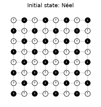
# The initial Néel state: |1⟩ (black, ↓) on odd sites, |0⟩ (white, ↑) on even sites

fig, ax = plt.subplots(figsize=(4, 4.4))
for i, j in all_bonds:
    ax.plot(
        [i % side, j % side],
        [i // side, j // side],
        color="0.75",
        lw=1,
        zorder=0,
    )
for q in range(side * side):
    x, y = q % side, q // side
    excited = (x + y) % 2 == 1
    ax.scatter(
        x,
        y,
        s=150,
        color="black" if excited else "white",
        edgecolor="black",
        zorder=2,
    )
    ax.text(
        x,
        y,
        "↓" if excited else "↑",
        ha="center",
        va="center",
        fontsize=7,
        color="white" if excited else "black",
        zorder=3,
    )
ax.set_aspect("equal")
ax.set_xlim(-1, side)
ax.set_ylim(side, -1)
ax.axis("off")
ax.set_title("Initial state: Néel", fontsize=13)
plt.show()
# actual circuit construction:
def heisenberg_floquet_circuit(
    num_cols, num_rows, coupling, num_cycles, disorder, measure=True
):
    num_qubits = num_cols * num_rows
    circuit = QuantumCircuit(num_qubits)
    neel_state(circuit, num_cols, num_rows, list(range(num_qubits)))
    cycle = QuantumCircuit(num_qubits)
    for sublayer in disorder:
        for (i, j), (h_i, h_j) in sublayer:
            heisenberg_gate(cycle, coupling, i, j, h_i, h_j)
    for _ in range(num_cycles):
        circuit.compose(cycle, inplace=True)
    if measure:
        circuit.measure_all()
    return circuit
Isang halimbawang
Gumagamit ang mga simulation ng na lattice na may dalawang cycle, at ang mga coupling na na pinag-aralan sa paper. Isang set ng mga field ang ginagamit muli para sa bawat coupling.
# simulation parameters:
num_cols = num_rows = 4
num_qubits = num_cols * num_rows
num_cycles = 2
couplings = (
    np.array([0.005, 0.01, 0.02, 0.03, 0.04, 0.05, 0.06, 0.08, 0.10, 0.125])
    * np.pi
)
disorder = sample_disorder(num_cols, num_rows, np.random.default_rng(42))

# circuit construction:
logical_circuits = [
    heisenberg_floquet_circuit(
        num_cols, num_rows, coupling, num_cycles, disorder
    )
    for coupling in couplings
]
logical_circuits[5].draw(output="mpl", fold=-1)

# transpiling the circuit:
pass_manager = generate_preset_pass_manager(
    optimization_level=3,
    basis_gates=["cz", "rz", "sx", "x"],
    seed_transpiler=7,
)
circuits = [pass_manager.run(circuit) for circuit in logical_circuits]

def two_qubit_stats(circuit):
    count = sum(1 for inst in circuit.data if inst.operation.num_qubits == 2)
    depth = circuit.depth(lambda inst: inst.operation.num_qubits == 2)
    return count, depth

stats = {two_qubit_stats(circuit) for circuit in circuits}
assert len(stats) == 1, "the CZ structure should not depend on J"
num_cz, depth = stats.pop()
print(
    f"{num_qubits} qubits: {num_cz} CZ gates in {depth} layers, for every coupling"
)
circuits[5].draw("mpl", fold=-1, scale=0.4)
16 qubits: 144 CZ gates in 24 layers, for every coupling

Hindi kailangan ng matalinong compiler, dahil ang mga Circuit (at experiment) ay dinisenyo para sa IBM Nighthawk.
I-simulate ang na lattice
Para sa na lattice, magagawa mo ang pareho: kalkulahin ang eksaktong state sa bawat coupling, at i-sample ang bawat Circuit gamit ang 10,000 shot, tulad ng gagawin ng isang experiment. Naka-store ang mga shot na may hugis (mga batch, mga shot, mga Qubit), ang parehong layout ng mga randomization sa data ng hardware. Dito, isang batch ang binubuo ng lahat ng 10,000 shot, kaya walang idinadagdag na shot noise ang bootstrap sa mga batch, at ang spread lang sa pagitan ng mga marginal na posisyon ang ipinapakita ng mga error bar sa susunod na plot.
exact_states = [
    Statevector(
        heisenberg_floquet_circuit(
            num_cols, num_rows, c, num_cycles, disorder, measure=False
        )
    )
    for c in couplings
]

shots = 10_000
results = (
    StatevectorSampler(default_shots=shots, seed=1234).run(circuits).result()
)

# the output of the simulation for the 10 couplings
bits = [
    result.data.meas.to_bool_array(order="little").reshape(
        1, 10_000, num_qubits
    )
    for result in results
]

print(bits[0])
[[[False  True False ... False  True False]
  [False  True False ... False  True False]
  [False  True False ... False  True False]
  ...
  [False  True False ... False  True False]
  [False  True False ... False  True False]
  [False  True False ... False  True False]]]
2. Ano ang susukatin at paano ito tantiyahin
Ang IPR at ang collision entropy
Para sa isang marginal na ng Qubit na may bitstring distribution na , ang dapat tantiyahin ay ang inverse participation ratio (IPR) ng marginal distribution, at mula rito ang collision entropy:
Ang ay ang probabilidad din na magkasundo ang dalawang shot sa marginal. Ang product state ay may , at ang random state ay may , kaya umaakyat ang mula 0 hanggang halos bit habang nagiging random ang marginal.
Estimator 1: bilangin ang mga pares ng shot
Question. Paano mo tatantiyahin ang dami na ito mula sa iyong mga shot?
Sagot
Kinukwenta ng naive na estimator ang bawat mula sa mga shot bilang , pagkatapos ay sinusuma ang . Biased ang estimator na ito.
Binibilang ng ang bawat shot bilang kasundo ang sarili nito, na nagtataas sa tantiya: sa karaniwan, ibinibigay nito ang sa halip na . Dahil ang ay ang probabilidad na magkasundo ang dalawang shot, bilangin lang ang mga pares ng magkaibang shot:
Unbiased ito, at ito ang kinukwenta ng ipr_from_shots sa ibaba.
# IPR expectation values:

# refactor this function cause it does not scale
def ipr_from_shots(bits):
    # Pair-counting estimate of the IPR of a marginal: the fraction of pairs of different shots
    # that agree on it. bits holds the marginal's qubits only, with shape (randomizations, shots,
    # qubits), and all randomizations are pooled.
    n = bits.shape[-1]
    outcomes = bits @ 2 ** np.arange(
        n
    )  # each shot's marginal bitstring, read as an integer
    counts = np.bincount(outcomes.ravel())  # how often each outcome occurs
    total = counts.sum()
    return float((counts * (counts - 1)).sum() / (total * (total - 1)))

def collision_entropy(ipr):
    return -np.log2(ipr)
Estimator 2: Parseval expansion
Maisusulat din ang IPR sa pamamagitan ng mga parity na ng lahat ng hindi walang laman na subset na ng marginal:
Mahalaga ang anyong ito dahil gumagana ang mga paraan ng error mitigation tulad ng PEA sa mga expectation value, hindi sa mga probabilidad. Isang Qubit: Ang mga probabilidad ng outcome ay at , kaya
Isang na marginal: Kapag may label na ang mga Qubit nito, may parity ang marginal: 4 na single qubit, 6 na pares, 4 na triple, at ang buong marginal, kaya
def parity_supports(patch):
    # All nonempty subsets S of the marginal
    return sorted(
        [
            tuple(q for k, q in enumerate(patch) if mask & (1 << k))
            for mask in range(1, 1 << len(patch))
        ],
        key=len,
    )

def parity_expectation_values(bits, supports):
    # Shot-averaged <Z_S> for every support, per randomization
    signs = 1 - 2 * bits.astype(np.int8)
    return np.stack(
        [signs[..., list(s)].prod(axis=-1).mean(axis=-1) for s in supports],
        axis=-1,
    )

# Example: the parities of a 3-qubit marginal made of lattice qubits 5, 6, and 9
print(parity_supports([5, 6, 9]))
print(f"A 3×3 marginal has {len(parity_supports(range(9)))} parities")
[(5,), (6,), (9,), (5, 6), (5, 9), (6, 9), (5, 6, 9)]
A 3×3 marginal has 511 parities
Average sa mga marginal
Mga karagdagang kapaki-pakinabang na function: mga halaga ng Haar, pagpili ng mga marginal, bootstrapping, at pag-aaverage.
# functions for the Haar values on plots:
def haar_ipr(num_patch, num_qubits):
    # Mean IPR of a marginal for Haar-random states in the sector with num_qubits // 2 ones
    weight = num_qubits // 2
    dimension = comb(num_qubits, weight)
    total = 0
    for k in range(num_patch + 1):  # k ones on the marginal
        rest = (
            comb(num_qubits - num_patch, weight - k) if weight - k >= 0 else 0
        )
        total += comb(num_patch, k) * rest * (rest + 1)
    return total / (dimension * (dimension + 1))

def haar_entropy(num_patch, num_qubits):
    return collision_entropy(haar_ipr(num_patch, num_qubits))

# definitions of positions in the lattice:
def patch_qubits(anchor, shape, num_cols):
    # Lattice indices of a rectangular marginal with its top-left corner at anchor
    (x0, y0), (width, height) = anchor, shape
    return [
        (y0 + dy) * num_cols + (x0 + dx)
        for dy in range(height)
        for dx in range(width)
    ]

def all_positions(shape, num_cols, num_rows):
    # Every placement of a (width, height) marginal on the lattice
    width, height = shape
    return [
        patch_qubits((x, y), shape, num_cols)
        for y in range(num_rows - height + 1)
        for x in range(num_cols - width + 1)
    ]

# bootstrapping for error bars:
bootstrap_rng = np.random.default_rng(0)

def bootstrap_error(statistic, *samples, axis=0, num_resamples=50):
    # Shot noise of a statistic, from resampling the randomizations (along axis of every
    # sample) with replacement
    values = []
    for _ in range(num_resamples):
        resampled = [
            np.take(
                x,
                bootstrap_rng.integers(0, x.shape[axis], x.shape[axis]),
                axis=axis,
            )
            for x in samples
        ]
        values.append(statistic(*resampled))
    return float(np.std(values, ddof=1))

# averaging the ipr over marginals:
def average_ipr(iprs, shot_errors):
    # iprs and shot_errors have shape (positions, couplings). The mean IPR over positions, and its
    # error: the spread between positions plus the shot noise of each (law of total variance)
    iprs, shot_errors = np.asarray(iprs), np.asarray(shot_errors)
    count = len(iprs)
    variance = (
        iprs.var(axis=0, ddof=1) / count
        + (shot_errors**2).sum(axis=0) / count**2
    )
    return iprs.mean(axis=0), np.sqrt(variance)
# Calculating exact simulation entropies:
patch_shapes = {
    "1×1": (1, 1),
    "1×2": (2, 1),
    "2×2": (2, 2),
    "2×3": (3, 2),
    "3×3": (3, 3),
}

# calculate the exact entropies:
sim_positions = {
    label: all_positions(shape, num_cols, num_rows)
    for label, shape in patch_shapes.items()
}
exact_iprs = {  # shape (positions, couplings)
    label: np.array(
        [
            [(s.probabilities(qargs=q) ** 2).sum() for s in exact_states]
            for q in qubit_lists
        ]
    )
    for label, qubit_lists in sim_positions.items()
}
exact_entropies = {
    label: collision_entropy(v.mean(axis=0))
    for label, v in exact_iprs.items()
}

# Average IPR of every shape over its positions, from the sampled shots, then the entropy
iprs_from_shots = {}  # per shape: average IPR and its error, at every coupling
entropies_from_shots = {}  # per shape: average entropy and its error, at every coupling
for label, qubit_lists in sim_positions.items():
    iprs = [[ipr_from_shots(b[:, :, q]) for b in bits] for q in qubit_lists]

    # bootstrapping over subsampling for error bars:
    errors = [
        [bootstrap_error(ipr_from_shots, b[:, :, q]) for b in bits]
        for q in qubit_lists
    ]
    ipr, ipr_error = average_ipr(iprs, errors)
    iprs_from_shots[label] = (ipr, ipr_error)
    entropies_from_shots[label] = (
        collision_entropy(ipr),
        ipr_error / (ipr * np.log(2)),
    )
# Now plot the average IPR on the left, and the same averages as entropies on the right
colors = plt.cm.plasma(np.linspace(0.05, 0.8, len(patch_shapes)))
fig, (ax_ipr, ax_entropy) = plt.subplots(1, 2, figsize=(12.8, 4.2))
for (label, qubit_lists), color in zip(sim_positions.items(), colors):
    n = len(qubit_lists[0])
    ipr, ipr_error = iprs_from_shots[label]
    entropy, entropy_error = entropies_from_shots[label]
    # Left: the average IPR, with its exact value and its random-state value
    ax_ipr.axhline(haar_ipr(n, num_qubits), color=color, ls="dashdot", lw=0.9)
    ax_ipr.plot(
        couplings / np.pi, exact_iprs[label].mean(axis=0), color=color
    )
    ax_ipr.errorbar(
        couplings / np.pi,
        ipr,
        yerr=ipr_error,
        fmt="o",
        color=color,
        mec="white",
        ms=7,
        capsize=3,
        label=f"{label} ({len(qubit_lists)} positions)",
    )
    # Right: the average collision entropy
    ax_entropy.axhline(
        haar_entropy(n, num_qubits), color=color, ls="dashdot", lw=0.9
    )
    ax_entropy.plot(couplings / np.pi, exact_entropies[label], color=color)
    ax_entropy.errorbar(
        couplings / np.pi,
        entropy,
        yerr=entropy_error,
        fmt="o",
        color=color,
        mec="white",
        ms=7,
        capsize=3,
        label=f"{label} ({len(qubit_lists)} positions)",
    )
ax_ipr.set_yscale("log")
ax_ipr.set_ylabel("Average IPR")
ax_entropy.set_ylabel("Average collision entropy (bits)")
for ax in (ax_ipr, ax_entropy):
    ax.set_xlabel("Coupling $J/\\pi$")
fig.suptitle("Exact (lines) and sampled (dots), 4×4 lattice, 2 cycles")
ax_entropy.legend(title="Marginal", loc="upper left")
fig.tight_layout()
plt.show()
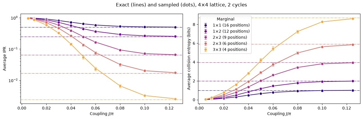
Ang bawat hugis ng marginal ay maayos na tumataas papunta sa halaga nito sa random na state, at ang mas malalaking marginal ay umaabot doon sa mas malalaking .
3. Noise, at paano ito aalisin
Isang noisy na simulation
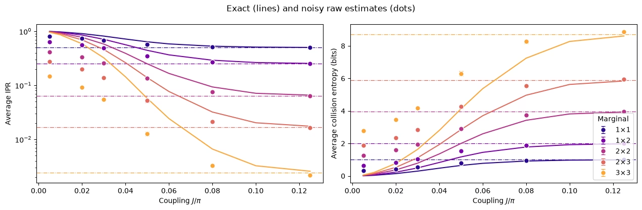
Ngayon, magdagdag ng noise: 1% two-qubit depolarizing noise sa bawat CZ gate at 3% readout error sa bawat qubit, na sinample gamit ang Qiskit Aer sampler. Dahil may 144 CZ gate sa circuit, mas kaunti ito kaysa sa noise na nararanasan ng 8×8 hardware circuit, pero sapat na para makita ang epekto nito. Gumagamit ang simulation ng anim na coupling at tig-4,000 shot, at tumatagal nang mga 1.5 minuto.
Tanong. Bago mo ito patakbuhin: magmumukha bang mas thermalized o mas hindi thermalized ang system dahil sa noise?
Sagot
Mas thermalized. Ginugulo ng noise ang mga resulta, kaya napupunta sa uniform ang bawat marginal distribution, bumababa ang raw na IPR, at tumataas ang entropy. Kapag walang mitigation, magmumukhang may thermalization ang noise kahit wala naman, at masyadong maaga ang labas ng mga crossover.
# define the noise model

noise_model = NoiseModel()
# two qubit depolarizing noise:
noise_model.add_all_qubit_quantum_error(depolarizing_error(0.01, 2), ["cz"])
# symmetric readout noise:
noise_model.add_all_qubit_readout_error(
    ReadoutError([[0.97, 0.03], [0.03, 0.97]])
)

# simulation is done using trajectories
noisy_sampler = AerSampler(
    default_shots=4000,
    seed=1,
    options={"backend_options": {"noise_model": noise_model}},
)

# choose a subset of J values for speed:
noisy_indices = [
    0,
    2,
    3,
    5,
    7,
    9,
]  # J/π = 0.005, 0.02, 0.03, 0.05, 0.08, 0.125
noisy_results = noisy_sampler.run(
    [circuits[k] for k in noisy_indices]
).result()

# No twirling here, so the 20 "randomizations" are just batches of 200 shots
noisy_bits = {
    k: result.data.meas.to_bool_array(order="little").reshape(
        20, 200, num_qubits
    )
    for k, result in zip(noisy_indices, noisy_results)
}
# Calculating noisy entropies

# Average IPR of every shape over its positions, from the noisy shots, then the entropy
noisy_iprs = {}  # per shape: average IPR and its error, at every noisy coupling
noisy_entropies = {}  # per shape: average entropy and its error, at every noisy coupling
for label, qubit_lists in sim_positions.items():
    iprs = [
        [ipr_from_shots(noisy_bits[k][:, :, q]) for k in noisy_indices]
        for q in qubit_lists
    ]

    # bootstrapping over subsampling for error bars:
    errors = [
        [
            bootstrap_error(ipr_from_shots, noisy_bits[k][:, :, q])
            for k in noisy_indices
        ]
        for q in qubit_lists
    ]
    ipr, ipr_error = average_ipr(iprs, errors)
    noisy_iprs[label] = (ipr, ipr_error)
    noisy_entropies[label] = (
        collision_entropy(ipr),
        ipr_error / (ipr * np.log(2)),
    )
fig, (ax_ipr, ax_entropy) = plt.subplots(1, 2, figsize=(12.8, 4.2))
for (label, qubit_lists), color in zip(sim_positions.items(), colors):
    n = len(qubit_lists[0])
    ipr, ipr_error = noisy_iprs[label]
    entropy, entropy_error = noisy_entropies[label]
    # Left: the average IPR, with its exact value and its random-state value
    ax_ipr.axhline(haar_ipr(n, num_qubits), color=color, ls="dashdot", lw=0.9)
    ax_ipr.plot(
        couplings / np.pi, exact_iprs[label].mean(axis=0), color=color
    )
    ax_ipr.errorbar(
        couplings[noisy_indices] / np.pi,
        ipr,
        yerr=ipr_error,
        fmt="o",
        color=color,
        mec="white",
        ms=7,
        capsize=3,
        label=label,
    )
    # Right: the same averages as entropies
    ax_entropy.axhline(
        haar_entropy(n, num_qubits), color=color, ls="dashdot", lw=0.9
    )
    ax_entropy.plot(couplings / np.pi, exact_entropies[label], color=color)
    ax_entropy.errorbar(
        couplings[noisy_indices] / np.pi,
        entropy,
        yerr=entropy_error,
        fmt="o",
        color=color,
        mec="white",
        ms=7,
        capsize=3,
        label=label,
    )
ax_ipr.set_yscale("log")
ax_ipr.set_ylabel("Average IPR")
ax_entropy.set_ylabel("Average collision entropy (bits)")
for ax in (ax_ipr, ax_entropy):
    ax.set_xlabel("Coupling $J/\\pi$")
fig.suptitle("Exact (lines) and noisy raw estimates (dots)")
ax_entropy.legend(title="Marginal", loc="lower right")
fig.tight_layout()
plt.show()
Brainstorm: paano mo ito aalisin?
Iminumungkahing paraan
Sa maliit na , halos hindi entangled ang state, kaya madali sa classical na kalkulahin ang ideal na sagot doon, kahit para sa 64 qubit. Ibig sabihin, masusukat ang epekto ng noise sa isang maliit na calibration coupling na at magagamit ito para itama ang lahat ng ibang coupling. May dalawang natural na paraan para dito, na tinatawag na low-entanglement calibration (LEC):
LEC sa IPR. I-rescale ang sobra ng IPR kumpara sa halaga nito para sa uniform na distribution, , gamit ang isang factor kada marginal:
LEC sa mga expectation value ng . I-rescale ang bawat parity ng marginal gamit ang sarili nitong factor, at buuin muli ang IPR gamit ang Parseval formula:
Sa code, ang bawat squared na rescaled parity ay dine-debias sa pamamagitan ng pagbabawas ng variance nito, tulad ng sa seksyon 2.
Pareho lang ang dalawa kung ang bawat ay katumbas ng .
Question. What are the pros and cons of these methods?
Sagot
Pros
-
Mura: walang karagdagang data na kailangan mula sa device, classical simulation lang sa .
-
Ginagamit ang istruktura ng circuit: hindi nagbabago sa ang lalim ng circuit at ang mga CZ layer, kaya ang noise sa ay kapareho ng noise sa bawat ibang .
Cons
- Ipinapalagay na hindi nakadepende sa ang epekto ng noise sa mga observable: pareho ang noise mismo, pero maaaring magbago ang paraan ng pagpapahina nito sa IPR o sa bawat habang lumalaki ang .
Parehong paraan sa noisy na simulation
# function to mitigate the IPR signal:
def mitigate_ipr_w_lec(
    ipr_raw, ipr_raw_calibration, ipr_ideal_calibration, num_patch
):
    # LEC on the IPR: one factor R0 for the excess over the uniform value
    uniform = 2.0**-num_patch
    factor = (ipr_ideal_calibration - uniform) / (
        ipr_raw_calibration - uniform
    )
    return uniform + factor * (ipr_raw - uniform)

# function used to calculate the target <Z> expectation values
def parities_from_probabilities(probabilities):
    # Ideal <Z_S> from a marginal distribution, in parity_supports order: subsets
    # by size, and in bitmask order within each size
    outcomes = np.arange(len(probabilities))
    masks = np.array(sorted(range(1, len(probabilities)), key=int.bit_count))
    signs = (-1.0) ** np.bitwise_count(outcomes[:, None] & masks[None, :])
    return np.asarray(probabilities) @ signs

# calculate boosting factors:
def lec_z_factors(calibration_parities, ideal_parities):
    # LEC on <Z>: one factor r_S per parity, from data with shape (randomizations, supports).
    return ideal_parities / calibration_parities.mean(axis=0)

# function to mitigate the IPR from <Z> expectation values:
def mitigate_ipr_w_lec_on_parities(
    parities, calibration_parities, ideal_calibration_parities, num_patch
):
    # LEC on <Z>: rescale each parity by its factor r_S = ideal / raw at J0, then rebuild the IPR
    # with Parseval. parities and calibration_parities have shape (randomizations, supports).
    # Each squared, rescaled parity is debiased by subtracting its variance, which to first
    # order combines the shot noise at J. The shot noise of r_S from J0 is omitted; including it
    # does not change the results.
    factors = lec_z_factors(calibration_parities, ideal_calibration_parities)
    mean = parities.mean(axis=0)  # mean over the twirling instances
    variance = parities.var(axis=0, ddof=1) / len(
        parities
    )  # variance of the mean
    rescaled = factors * mean
    rescaled_variance = factors**2 * variance
    return float((1 + np.sum(rescaled**2 - rescaled_variance)) / 2**num_patch)
def lec_estimates(patch_bits, parities, ideal, calibration, num_patch):
    # LEC on the IPR and on <Z> for one marginal position, at every coupling: values and shot
    # noise. patch_bits (the bits of the marginal only) and parities are per coupling, with
    # randomizations first.
    q_ideal = (ideal**2).sum()
    ideal_parities = parities_from_probabilities(ideal)

    def ipr_statistic(b, c):
        return mitigate_ipr_w_lec(
            ipr_from_shots(b), ipr_from_shots(c), q_ideal, num_patch
        )

    def z_statistic(p, c):
        return mitigate_ipr_w_lec_on_parities(p, c, ideal_parities, num_patch)

    values = {"LEC on IPR": [], "LEC on ⟨Z⟩": []}
    errors = {"LEC on IPR": [], "LEC on ⟨Z⟩": []}
    for k in range(len(patch_bits)):
        if (
            k == calibration
        ):  # both match the ideal value at J0 by construction
            for method in values:
                values[method].append(q_ideal)
                errors[method].append(0.0)
            continue
        values["LEC on IPR"].append(
            ipr_statistic(patch_bits[k], patch_bits[calibration])
        )
        errors["LEC on IPR"].append(
            bootstrap_error(
                ipr_statistic, patch_bits[k], patch_bits[calibration]
            )
        )
        values["LEC on ⟨Z⟩"].append(
            z_statistic(parities[k], parities[calibration])
        )
        errors["LEC on ⟨Z⟩"].append(
            bootstrap_error(z_statistic, parities[k], parities[calibration])
        )
    return values, errors

# getting all the data:
calibration_index = 0  # index of J0 = 0.005π in noisy_indices
mitigated = {
    "LEC on IPR": {},
    "LEC on ⟨Z⟩": {},
}  # per shape: (values, errors), each (positions, couplings)
for label, qubit_lists in sim_positions.items():
    n = len(qubit_lists[0])
    per_position = []
    for qubits in qubit_lists:
        supports = parity_supports(qubits)
        parities = [
            parity_expectation_values(noisy_bits[k], supports)
            for k in noisy_indices
        ]
        patch_bits = [noisy_bits[k][:, :, qubits] for k in noisy_indices]
        ideal = exact_states[noisy_indices[calibration_index]].probabilities(
            qargs=qubits
        )
        per_position.append(
            lec_estimates(patch_bits, parities, ideal, calibration_index, n)
        )
    for method in mitigated:
        mitigated[method][label] = (
            [p[0][method] for p in per_position],
            [p[1][method] for p in per_position],
        )

# Average over positions, then the entropy, for both methods
mitigated_entropies = {
    method: {} for method in mitigated
}  # per method and shape: entropy and its error
for method, by_shape in mitigated.items():
    for label, (values, errors) in by_shape.items():
        ipr, ipr_error = average_ipr(values, errors)
        mitigated_entropies[method][label] = (
            collision_entropy(ipr),
            ipr_error / (ipr * np.log(2)),
        )  # log here comes from error propagation
# Plot the data mitigated with both methods:

fig, axes = plt.subplots(1, 2, figsize=(12.8, 4.2), sharey=True)
for ax, (method, by_shape) in zip(axes, mitigated_entropies.items()):
    for (label, qubit_lists), color in zip(sim_positions.items(), colors):
        entropy, error = by_shape[label]
        ax.axhline(
            haar_entropy(len(qubit_lists[0]), num_qubits),
            color=color,
            ls="dashdot",
            lw=0.9,
        )
        ax.plot(couplings / np.pi, exact_entropies[label], color=color)
        ax.errorbar(
            couplings[noisy_indices] / np.pi,
            entropy,
            yerr=error,
            fmt="o",
            color=color,
            mec="white",
            ms=7,
            capsize=3,
            label=label,
        )
    ax.set_title(f"{method} (lines: exact)")
    ax.set_xlabel("Coupling $J/\\pi$")
axes[0].set_ylabel("Average collision entropy (bits)")
axes[0].legend(title="Marginal", loc="lower right")
fig.tight_layout()
plt.show()

# add the noisy data here too
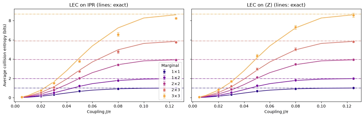
Inaalis ng parehong paraan ang karamihan sa pinsala: masyadong random ang mga raw na estimate sa nakaraang plot, at sinusundan ng mga na-mitigate ang mga eksaktong curve. Lumalabas ang mga pagkakaiba sa mas malalaking marginal.
Sa maliliit na marginal, gumagana ang parehong paraan. Para sa na marginal, mas malapit nang malinaw ang LEC sa .
Bakit kulang ang entropy sa LEC sa IPR. Ang kulang na entropy ay nangangahulugang masyadong malaki ang IPR: pinalalaki ito nang sobra ng LEC sa IPR. Ipinapalagay nito na pinapahina ng noise ang kontribusyon ng bawat sa IPR gamit ang parehong factor. Sa , malapit sa ang bawat , kaya pantay ang kontribusyon ng lahat ng string, at karamihan sa mga string ay may katamtamang weight: sa 511 string ng isang na marginal, 252 ang may weight na 4 o 5, at siyam lang ang may weight na 1. Mas pinapahina ng noise ang isang string kapag mas mataas ang weight nito (ang readout error lang ay pinapahina na ang isang string na may weight na ng ), kaya ang nag-iisang factor na ay pangunahing itinakda ng pagpapahina sa mga string na katamtaman ang weight. Habang lumalaki ang , pinakamabilis na nawawala ang mga na mas mataas ang weight, at ang IPR ay lalong dinadala ng mga string na mababa ang weight, na mas kaunti ang pagpapahina ng noise. Ang pagpapalakas sa mga ito gamit ang factor na pangunahing natutunan mula sa mas pinahinang mga string ay sobrang nagpapalaki sa IPR. Lumalaki ang epektong ito kasabay ng laki ng marginal, dahil mas malawak ang saklaw ng weight ng mas malaking marginal. Pinakamalaki ito sa katamtamang , pagkatapos lumipat ang halo ng mga string pero mahalaga pa rin ang sobra ng IPR sa uniform na halaga nito.
Bakit kabaligtaran ang mali ng LEC sa . Nire-rescale nito ang bawat string gamit ang sarili nitong factor, kaya hindi ito apektado ng paglipat sa pagitan ng mga weight. Ipinapalagay lang nito na napapanatili ng bawat string ang pagpapahina nito sa . Habang lumalaki ang , kumakalat ang bawat sa mga operator na mas mataas ang weight, na mas maraming noise ang nakukuha kaysa sa , kaya bahagyang kulang ang pagtatama ng mga factor at bahagyang masyadong mataas ang lumalabas na entropy.
Kaya ang prediksyon na susubukan sa hardware ay: habang mas malaki ang marginal, mas dapat manalo ang LEC sa . Sa hardware, mas malakas ang noise at hindi ito kilalang anyo.
4. Patakbuhin nang malakihan
Ang hardware experiment ay nagpapatakbo ng na lattice na may apat na cycle: 64 qubit at 1,344 CZ gate sa 48 layer, sa siyam na coupling. Limang bagay ang nagbabago kumpara sa simulation:
-
Kailangang matutunan ang noise, na gumagana lang kung nakapirmi ang mga CZ layer.
-
Ginagawa ng Twirling na Pauli channel ang noise ng bawat layer, na maaaring matutunan at palakasin.
-
Pinoprotektahan ng Dynamical decoupling (DD) ang mga idle na qubit.
-
Ang Noise amplification para sa PEA ay tumatakbo sa parehong job ng pangunahing data.
-
Ang mga MPS simulation sa maliit na ang nagbibigay ng mga classical na reference para sa error mitigation na nakabatay sa LEC.
Ang mga cell na nangangailangan ng backend ay tumatakbo lang kapag ang RUN_ON_HARDWARE ay True. Maaaring patakbuhin muli ang mga MPS simulation kapag ang COMPUTE_MPS_REFERENCES ay nakatakda sa True. Ang iba pang mga cell ay tumatakbo dito.
# hardware run parameters:
num_cols_hw = num_rows_hw = 8
num_qubits_hw = num_cols_hw * num_rows_hw
num_cycles_hw = 4
couplings_hw = (
    np.array([0.005, 0.01, 0.02, 0.03, 0.05, 0.07, 0.09, 0.11, 0.125]) * np.pi
)
calibration_hw = 0  # J0 = 0.005π
disorder_hw = sample_disorder(
    num_cols_hw, num_rows_hw, np.random.default_rng(7)
)

# if running PEA:
noise_factors = np.array([1.0, 1.5, 2.0])  # PEA noise-amplification factors
Mga nakapirming CZ layer
def compile_by_sublayer(
    num_cols,
    num_rows,
    coupling,
    num_cycles,
    disorder,
    pass_manager,
    layout=None,
    num_physical_qubits=None,
):
    # Compile each sublayer once and repeat it with barriers, so the CZ layers are the
    # same in every cycle and at every coupling. The registers are named explicitly
    # because register names enter Samplomatic's box hashes. Bits land in lattice order.
    num_qubits = num_cols * num_rows
    if layout is None:
        layout, num_physical_qubits = list(range(num_qubits)), num_qubits
    blocks = []
    for sublayer in disorder:
        block = QuantumCircuit(num_qubits)
        for (i, j), (h_i, h_j) in sublayer:
            heisenberg_gate(block, coupling, i, j, h_i, h_j)
        blocks.append(pass_manager.run(block))
    circuit = QuantumCircuit(
        QuantumRegister(num_physical_qubits, "q"),
        ClassicalRegister(num_qubits, "meas"),
    )
    neel_state(circuit, num_cols, num_rows, layout)
    for _ in range(num_cycles):
        for block in blocks:
            circuit.compose(block, inplace=True)
            circuit.barrier(layout)
    circuit.measure(layout, range(num_qubits))
    return circuit
Mga box para sa noise learning
Pagkatapos, ang Samplomatic boxing pass manager ay naghahati ng bawat circuit sa mga box: isa para sa bawat CZ layer at isa para sa mga measurement. May dalang reference ang bawat box sa noise model na kailangan nito, kaya masusuri mo kung pareho ang mga box ng lahat ng coupling. Ginagawa ito ng susunod na cell para sa mga na circuit ng hardware run, na na-compile sa mga CZ gate nang walang backend, at inililimbag ang mga box na iku-characterize ng noise learning.
from samplomatic import build
from samplomatic.transpiler import generate_boxing_pass_manager
from samplomatic.utils import find_unique_box_instructions

boxing_pass_manager = generate_boxing_pass_manager(
    enable_gates=True,  # twirl the CZ layers
    enable_measures=True,  # twirl the measurements
    inject_noise_targets="gates",  # PEA amplifies the noise of the CZ layers only
    inject_noise_strategy="uniform_modification",
)

def noise_refs(boxed_circuit):
    return sorted(
        annotation.ref
        for box in find_unique_box_instructions(boxed_circuit.data)
        for annotation in box.operation.annotations
        if hasattr(annotation, "ref")
    )

# The 8x8 hardware circuits, compiled to CZ gates on the lattice qubits (no backend needed)
compiled_8x8 = [
    compile_by_sublayer(
        num_cols_hw, num_rows_hw, c, num_cycles_hw, disorder_hw, pass_manager
    )
    for c in couplings_hw
]
boxed_8x8 = [boxing_pass_manager.run(circuit) for circuit in compiled_8x8]
assert all(
    noise_refs(b) == noise_refs(boxed_8x8[0]) for b in boxed_8x8
), "layers differ between couplings"
num_cz, depth = two_qubit_stats(compiled_8x8[0])
print(
    f"{num_qubits_hw} qubits: {num_cz} CZ gates in {depth} layers, for every coupling"
)
for box in find_unique_box_instructions(boxed_8x8[0].data):
    ops = box.operation.blocks[0].count_ops()
    print(
        f"{box.operation.num_qubits}-qubit box: {ops.get('cz', 0)} CZ, {ops.get('measure', 0)} measurements"
    )
print(
    f"All {len(boxed_8x8)} couplings share these {len(find_unique_box_instructions(boxed_8x8[0].data))} boxes"
)
64 qubits: 1344 CZ gates in 48 layers, for every coupling
64-qubit box: 32 CZ, 0 measurements
64-qubit box: 24 CZ, 0 measurements
64-qubit box: 32 CZ, 0 measurements
64-qubit box: 24 CZ, 0 measurements
64-qubit box: 0 CZ, 64 measurements
All 9 couplings share these 5 boxes
I-twirl ang mga circuit
Sa bawat randomization, naglalagay ang Samplomatic ng mga random na Pauli gate bago ang bawat box at ng mga compensating na gate pagkatapos nito, na isinama sa mga katabing single-qubit gate. Kapag inaverage sa mga randomization, nagiging Pauli channel ang noise ng bawat layer, na maaaring matutunan ng NoiseLearnerV3 bilang sparse Pauli-Lindblad model at mapalakas ng hakbang ng PEA. Ang measurement twirling ay random na bumabaligtad ng mga bit bago ang readout. Binabawi ang mga pagbaligtad na ito sa software, na ginagawang simetriko ang readout noise at siyang batayan ng readout correction (TREX).
Ang hardware workflow
Piliin ang mga qubit, i-compile ang mga circuit, pagkatapos ay alamin ang noise at patakbuhin ang sweep. Naka-off ang mga cell na ito rito.
Piliin ang mga qubit. Kasya sa square grid ng Nighthawk ang na lattice nang walang SWAP gate. Binibigyan ng cell ng score ang bawat na parihaba ng grid ayon sa iniulat nitong CZ at readout error at kinukuha ang pinakamahusay.
def square_layouts(backend, side):
    # Every side x side rectangle of the square qubit grid that supports all bonds
    target = backend.target

    def has_cz(a, b):
        return (a, b) in target["cz"] or (b, a) in target["cz"]

    stride = next(
        s
        for s in (10, 12)
        if all(has_cz(q, q + s) for q in range(backend.num_qubits - s))
    )
    layouts = []
    for y0 in range(backend.num_qubits // stride - side + 1):
        for x0 in range(stride - side + 1):
            layout = [
                stride * (y0 + y) + x0 + x
                for y in range(side)
                for x in range(side)
            ]
            bonds = [
                bond
                for layer in brickwork_layers(side, side)
                for bond in layer
            ]
            if all(has_cz(layout[i], layout[j]) for i, j in bonds):
                layouts.append(((x0, y0), layout))
    return layouts

def layout_score(backend, layout, side, uses_per_bond):
    # Minus the summed log-fidelity of the bonds (each used uses_per_bond times) and readouts
    properties, target = backend.properties(), backend.target
    cz_errors = []
    for i, j in (
        bond for layer in brickwork_layers(side, side) for bond in layer
    ):
        pair = (
            (layout[i], layout[j])
            if (layout[i], layout[j]) in target["cz"]
            else (layout[j], layout[i])
        )
        cz_errors.append(properties.gate_error("cz", pair))
    readout_errors = [properties.readout_error(q) for q in layout]
    if max(cz_errors) >= 0.5 or max(readout_errors) >= 0.25:
        return np.inf  # an unusable qubit or bond
    return float(
        -uses_per_bond * np.log1p(-np.array(cz_errors)).sum()
        - np.log1p(-np.array(readout_errors)).sum()
    )

if RUN_ON_HARDWARE:
    from qiskit_ibm_runtime import QiskitRuntimeService

    def holds_lattice(backend):
        try:
            return bool(square_layouts(backend, num_cols_hw))
        except (KeyError, StopIteration):
            return False

    service = QiskitRuntimeService()
    candidates = [
        b
        for b in service.backends(operational=True, simulator=False)
        if holds_lattice(b)
    ]
    backend = min(candidates, key=lambda b: b.status().pending_jobs)
    score, origin, initial_layout = min(
        (
            layout_score(backend, layout, num_cols_hw, 3 * num_cycles_hw),
            origin,
            layout,
        )
        for origin, layout in square_layouts(backend, num_cols_hw)
    )
    print(f"{backend.name}: origin {origin}, score {score:.2f}")
I-compile. Parehong mga hakbang tulad ng nasa itaas sa mga napiling qubit, na sinusundan ng build, na ginagawang template circuit at isang samplex ang bawat boxed na circuit, ang recipe para sa pagguhit ng mga twirling gate at ng ini-inject na noise. Idinadagdag ang DD sa mga template.
if RUN_ON_HARDWARE:
    from qiskit_ibm_runtime.executor.dynamical_decoupling import (
        generate_dd_pass_manager,
    )
    from qiskit_ibm_runtime.options import DynamicalDecouplingOptions

    # PEA structure functions:
    target_pass_manager = generate_preset_pass_manager(
        target=backend.target,
        optimization_level=3,
        initial_layout=initial_layout,
        routing_method="none",
        seed_transpiler=7,
    )
    boxed_hw = [
        boxing_pass_manager.run(
            compile_by_sublayer(
                num_cols_hw,
                num_rows_hw,
                coupling,
                num_cycles_hw,
                disorder_hw,
                target_pass_manager,
                layout=initial_layout,
                num_physical_qubits=backend.num_qubits,
            )
        )
        for coupling in couplings_hw
    ]
    assert all(noise_refs(b) == noise_refs(boxed_hw[0]) for b in boxed_hw)
    unique_boxes_hw = find_unique_box_instructions(boxed_hw[0].data)

    # DD pass:
    dd_pass_manager = generate_dd_pass_manager(
        backend,
        DynamicalDecouplingOptions(
            enable=True,
            sequence_type="XY4",
            scheduling_method="alap",
            extra_slack_distribution="middle",
            skip_reset_qubits=False,
        ),
    )
    templates = []
    for circuit in boxed_hw:
        template, samplex = build(circuit)
        templates.append((dd_pass_manager.run(template), samplex))
Alamin ang noise at patakbuhin ang sweep. Isang NoiseLearnerV3 job ang natututo sa lahat ng limang box: isang Pauli-Lindblad model para sa bawat isa sa apat na CZ layer, at ang readout noise ng measurement box. Pagkatapos, hawak ng isang QuantumProgram ang lahat ng siyam na coupling. Nakakakuha ang bawat item ng template nito, samplex nito, mga natutunang noise model, at tatlong noise scale. Ang scale na 0 ay ang hindi pinalakas na data para sa parehong LEC method. Ang mga scale na 0.5 at 1 ay nagdadagdag ng 50% at 100% ng natutunang noise para sa PEA, na nag-e-extrapolate pabalik sa zero na noise. Gumagamit ito ng mga 40 segundo ng QPU time.
if RUN_ON_HARDWARE:
    from qiskit_ibm_runtime import Executor, NoiseLearnerV3, QuantumProgram

    # Learn the noise of the five boxes
    learner = NoiseLearnerV3(backend)
    learner.options.num_randomizations = 32
    learner.options.shots_per_randomization = 128
    # Up to 24 layer pairs, the depth of the 48-layer circuits
    learner.options.layer_pair_depths = [0, 1, 2, 4, 16, 24]
    learner_job = learner.run(unique_boxes_hw)
    print("Noise learning job:", learner_job.job_id())

    # Run the sweep, with the learned noise amplified by each of the noise factors
    noise_maps = learner_job.result().to_dict(
        instructions=unique_boxes_hw, require_refs=False
    )
    program = QuantumProgram(shots=200)
    for template, samplex in templates:
        program.append_samplex_item(
            template,
            samplex=samplex,
            samplex_arguments={
                "pauli_lindblad_maps": noise_maps,
                **{
                    f"noise_scales.{ref}": (noise_factors - 1).reshape(-1, 1)
                    for ref in noise_maps
                },
            },
            shape=(len(noise_factors), 200),  # noise scales x randomizations
        )
    executor_job = Executor(backend).run(program)
    print("Executor job:", executor_job.job_id())
    # Section 5 converts the results of these two jobs and saves them
5. Ang hardware data
Sinusuri ng seksyong ito kung paano gumagana ang mga naunang paraan sa totoong hardware data mula sa isang Nighthawk processor.
I-load ang run
Kapag ang RUN_ON_HARDWARE ay nakatakda sa True, kino-convert ng susunod na cell ang mga resulta ng dalawang job mula sa seksyon 4 at sine-save ang mga ito sa data/hardware_run_new.npz, sa parehong format ng naka-save na run, para maanalisa muli ang bagong run sa ibang pagkakataon. Kung hindi, nilo-load nito ang naka-save na run mula sa data/hardware_run.npz. Ang mga bit ay naka-pack sa kahabaan ng qubit axis para makatipid ng espasyo.
Kung mag-restart ang kernel habang tumatakbo ang mga job, huwag silang isumite muli. Patakbuhin muli ang mga cell bago ang huling tawag sa seksyon 4, tiyaking pareho ang mga napiling qubit, at itakda ang learner_job at executor_job sa service.job(job_id) gamit ang mga job ID na inilimbag sa seksyon 4.
if RUN_ON_HARDWARE:

    def unflip(item_result):
        # Undo the measurement twirling of an Executor item: flip back the bits that were flipped
        return item_result["meas"] ^ item_result["measurement_flips.meas"]

    learner_result = learner_job.result()
    raw_bits = [unflip(item) for item in executor_job.result()]

    # The learned readout map indexes the measured qubits in ascending physical order;
    # relabel it to lattice order
    measurement_box_index = next(
        k
        for k, box in enumerate(unique_boxes_hw)
        if "measure" in box.operation.blocks[0].count_ops()
    )
    measurement_box = next(
        inst
        for inst in boxed_hw[0].data
        if inst.operation.name == "box"
        and "measure" in inst.operation.blocks[0].count_ops()
    )
    measured = sorted(
        boxed_hw[0].find_bit(q).index for q in measurement_box.qubits
    )
    lattice_index = {physical: q for q, physical in enumerate(initial_layout)}
    readout_map = (
        learner_result[measurement_box_index]
        .to_pauli_lindblad_map()
        .apply_layout([lattice_index[p] for p in measured], num_qubits_hw)
    )

    # Save the run in the same format as the saved run, so it can be analyzed again later
    terms = readout_map.to_sparse_list()
    np.savez_compressed(
        "data/hardware_run_new.npz",
        bits=np.packbits(np.stack(raw_bits), axis=-1, bitorder="little"),
        labels=np.array([label for label, _, _ in terms]),
        indices=np.concatenate(
            [np.asarray(support) for _, support, _ in terms]
        ),
        rates=np.array([rate for _, _, rate in terms]),
        physical_qubits=np.array(initial_layout),
        couplings_over_pi=couplings_hw / np.pi,
        noise_factors=noise_factors,
    )
else:
    saved = np.load(
        "data/hardware_run.npz"
    )  # or data/hardware_run_new.npz, for a new run
    raw_bits = list(
        np.unpackbits(
            saved["bits"], axis=-1, count=num_qubits_hw, bitorder="little"
        ).astype(bool)
    )
    labels = [str(label) for label in saved["labels"]]
    indices = np.split(
        saved["indices"], np.cumsum([len(label) for label in labels])[:-1]
    )
    readout_map = PauliLindbladMap.from_sparse_list(
        list(zip(labels, indices, saved["rates"])), num_qubits_hw
    )

print(f"{len(raw_bits)} couplings, bits per coupling: {raw_bits[0].shape}")
print(
    f"Readout noise: {readout_map.num_terms} terms on {readout_map.num_qubits} qubits"
)
9 couplings, bits per coupling: (3, 200, 200, 64)
Readout noise: 64 terms on 64 qubits
Mga classical na reference
Kailangan ng parehong LEC method ang mga ideal na marginal distribution sa , at ang pagsubok sa mga ito ay nangangailangan ng mga ideal na halaga sa mga held-out na coupling na at . Galing ang mga ito sa mga matrix product state (MPS) simulation, na naka-save para sa bawat placement ng bawat hugis ng marginal sa lattice, tulad sa paper, at para sa bawat hindi nag-o-overlap na na block sa . Sa , nagko-converge ang mga ito sa bond dimension na . Sa at , gumagamit sila ng , at sa nagbabago pa rin sila nang hanggang mga 13% mula sa para sa mga na marginal, kaya ituring silang tinatayang halaga roon. Kinakalkula ang mga ito ng susunod na cell kung ang COMPUTE_MPS_REFERENCES ay True, na tumatagal nang mga 18 minuto, at kung hindi, nilo-load nito ang mga naka-save na resulta, na naka-key ayon sa coupling index, bond dimension, at marginal.
# Every placement of every shape on the 8x8 lattice
positions = {
    label: all_positions(shape, num_cols_hw, num_rows_hw)
    for label, shape in patch_shapes.items()
}
reference_settings = [
    (calibration_hw, 32),
    (calibration_hw, 64),
    (1, 128),
    (2, 64),
    (2, 128),
]  # (coupling, χ)

if COMPUTE_MPS_REFERENCES:

    def mps_patch_probabilities(coupling, patches, bond_dimension):
        # Distributions of the given marginals after the 8x8 circuit, from an MPS simulation
        simulator = AerSimulator(
            method="matrix_product_state",
            matrix_product_state_max_bond_dimension=bond_dimension,
            matrix_product_state_truncation_threshold=1e-12,
        )
        circuit = heisenberg_floquet_circuit(
            num_cols_hw,
            num_rows_hw,
            coupling,
            num_cycles_hw,
            disorder_hw,
            measure=False,
        )
        circuit = generate_preset_pass_manager(
            optimization_level=1, basis_gates=["cx", "u"], seed_transpiler=7
        ).run(circuit)
        for label, qubits in patches.items():
            circuit.save_probabilities(qubits, label=label)
        data = simulator.run(circuit, shots=1).result().data(0)
        return {label: np.asarray(data[label]) for label in patches}

    placements = {
        f"{label} {k}": qubits
        for label, patch_list in positions.items()
        for k, qubits in enumerate(patch_list)
    }
    tiles = {
        f"site {q}": [q] for q in range(num_qubits_hw)
    } | {  # for the lattice map at J0
        f"block {x},{y}": patch_qubits((2 * x, 2 * y), (2, 2), num_cols_hw)
        for y in range(num_rows_hw // 2)
        for x in range(num_cols_hw // 2)
    }
    computed = {}
    for index, chi in reference_settings:
        targets = (
            placements | tiles
            if (index, chi) == (calibration_hw, 64)
            else placements
        )
        for key, p in mps_patch_probabilities(
            couplings_hw[index], targets, chi
        ).items():
            computed[f"{index}/{chi}/{key}"] = p
    np.savez_compressed("data/mps_references_all.npz", **computed)
    saved = computed
else:
    saved = np.load("data/mps_references_all.npz")

references = {}  # (coupling index, bond dimension) -> {marginal key: distribution}
for name in saved:
    index, chi, key = name.split("/", 2)
    references.setdefault((int(index), int(chi)), {})[key] = saved[name]
Kalidad ng data: mga may sira na coupler / qubit
Una, tingnan ang pinakamababang coupling, , kung saan dapat malapit sa Néel checkerboard ang mga expectation value.
# <Z> of every site at J0: the MPS reference, and the hardware data at noise factor 1
z_reference = np.array(
    [
        parities_from_probabilities(
            references[(calibration_hw, 64)][f"site {q}"]
        )[0]
        for q in range(num_qubits_hw)
    ]
)
z_measured = 1 - 2 * raw_bits[calibration_hw][0].mean(axis=(0, 1))
fig, axes = plt.subplots(1, 2, figsize=(11, 4.6), layout="constrained")
fig.get_layout_engine().set(wspace=0.12)  # white space between the two panels
edges = np.arange(num_cols_hw + 1) - 0.5
for ax, values, title in zip(
    axes, (z_reference, z_measured), ("MPS reference", "Hardware")
):
    mesh = ax.pcolormesh(
        edges,
        edges,
        values.reshape(num_rows_hw, num_cols_hw),
        cmap="RdBu_r",
        vmin=-1,
        vmax=1,
        edgecolors="white",
    )
    ax.set_aspect("equal")
    ax.invert_yaxis()
    ax.set_xticks([])
    ax.set_yticks([])
    ax.set_title(
        f"{title}, $J_0 = {couplings_hw[calibration_hw] / np.pi:g}\\pi$"
    )
fig.colorbar(
    mesh, ax=axes, shrink=0.8, label=r"$\langle Z \rangle$ of each site"
)
plt.show()

Tanong. Kapag tiningnan ang hardware map, ano ang kapansin-pansin?
Sagot
Ang mga maputlang site, na halos nawala ang lahat ng signal kahit malapit sa Néel state ang state sa . Mahalaga ang mga ito dahil hinahati ng LEC sa anumang signal na natitira sa : ang qubit na halos walang signal ay nagbibigay ng napakalaki at maingay na correction factor, at ilang ganitong qubit ay maaaring mangibabaw sa bawat marginal na may kasamang mga ito.
Isang panuntunang data lang ang ginagamit: may sira ang isang qubit kung ang single-qubit IPR nito sa ay nasa loob ng mula sa , ang halaga para sa isang ganap na mixed na qubit. Dahil ang IPR ng isang qubit ay , tinutukoy nito ang mga qubit na may . Hindi isinasama sa ibaba ang mga marginal na may kasamang naka-flag na site.
site_iprs = np.array(
    [
        ipr_from_shots(raw_bits[calibration_hw][0][:, :, [q]])
        for q in range(num_qubits_hw)
    ]
)
# |IPR - 1/2| < 0.25**2 / 2 is the same as |<Z>| < 0.25
flagged = {
    q for q in range(num_qubits_hw) if abs(site_iprs[q] - 0.5) < 0.25**2 / 2
}
print(
    f"Median single-qubit IPR at J0: {np.median(site_iprs):.2f}; flagged lattice sites {sorted(flagged)}"
)
Median single-qubit IPR at J0: 0.77; flagged lattice sites [19, 24, 25, 27, 32]
Piliin ang mga marginal na i-aaverage
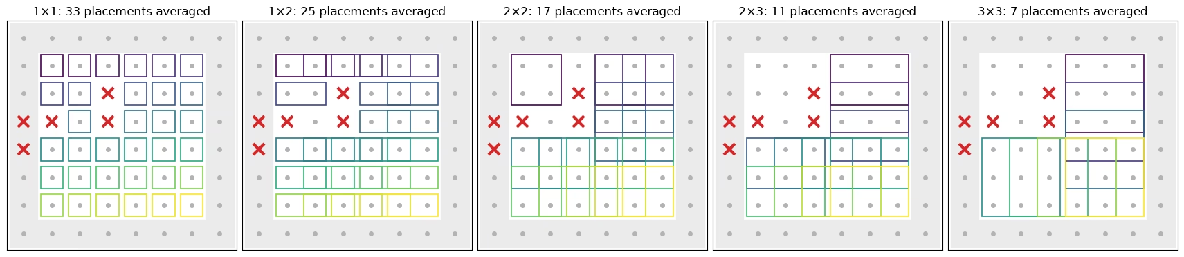
Ipinapakita ng susunod na cell kung aling mga placement ng bawat hugis ang pumapasok sa mga average sa ibaba: bawat placement sa bulk ng lattice na walang naka-flag na site (mga pulang krus). Hindi isinasama ang mga placement na dumidikit sa gilid (may shade). Mas kaunti ang bond ng mga edge qubit, kaya mas mabagal silang nag-scramble. Kapag inaverage nang mag-isa, nagko-crossover sila nang isang buong hakbang ng mamaya kaysa sa mga bulk placement, para sa bawat hugis at paraan. May sariling box ang bawat in-average na placement, na may kulay ayon sa placement.
def touches_edge(qubits):
    # Whether a placement includes a site on the edge of the lattice
    return any(
        q % num_cols_hw in (0, num_cols_hw - 1)
        or q // num_cols_hw in (0, num_rows_hw - 1)
        for q in qubits
    )

# The placements of each shape that enter the averages: in the bulk, and without a flagged site
kept_placements = {
    label: [
        k
        for k, qubits in enumerate(patch_list)
        if not touches_edge(qubits) and not set(qubits) & flagged
    ]
    for label, patch_list in positions.items()
}
placement_cmap = plt.get_cmap("viridis")
fig, axes = plt.subplots(
    1, len(positions), figsize=(17, 4.4), layout="constrained"
)
for ax, (label, patch_list) in zip(axes, positions.items()):
    width, height = patch_shapes[label]
    for q in range(num_qubits_hw):
        x, y = q % num_cols_hw, q // num_cols_hw
        if touches_edge([q]):  # shade the edge of the lattice
            ax.add_patch(
                plt.Rectangle(
                    (x - 0.5, y - 0.5), 1, 1, color="0.92", zorder=0
                )
            )
        ax.plot(x, y, "o", color="0.7", ms=4, zorder=1)
    kept = kept_placements[label]
    for i, k in enumerate(kept):
        qubits = patch_list[k]
        x0, y0 = (
            qubits[0] % num_cols_hw,
            qubits[0] // num_cols_hw,
        )  # top-left site of the placement
        ax.add_patch(
            plt.Rectangle(
                (x0 - 0.4, y0 - 0.4),
                width - 0.2,
                height - 0.2,
                fill=False,
                lw=1.2,
                ec=placement_cmap(i / max(len(kept) - 1, 1)),
                zorder=2,
            )
        )
    for q in flagged:
        ax.plot(
            q % num_cols_hw,
            q // num_cols_hw,
            "x",
            color="#d62728",
            ms=11,
            mew=3,
            zorder=3,
        )
    ax.set_xlim(-0.6, num_cols_hw - 0.4)
    ax.set_ylim(num_rows_hw - 0.4, -0.6)
    ax.set_aspect("equal")
    ax.set_xticks([])
    ax.set_yticks([])
    ax.set_title(f"{label}: {len(kept)} placements averaged")
plt.show()
PEA
Hindi na kailangan ng classical na reference ang ikatlong paraan. Para sa bawat parity, kunin ang mga halaga sa noise factor na 1, 1.5, at 2, hatiin sa natutunang readout damping (TREX), mag-fit ng exponential sa noise factor, at mag-extrapolate sa zero na noise. Ang mga parity na nagpapalit ng sign o halos zero ay nakakakuha ng straight-line fit. Ang pagbabawas ng variance ay nangangailangan ng maaasahang estimate nito, na madali para sa raw at rescaled na mga parity pero hindi para sa output ng nonlinear na fit na may clipping at mga fallback. Kaya gumagamit ang PEA ng isa pang karaniwang paraan para alisin ang bias ng isang square. I-extrapolate nang hiwalay ang bawat kalahati ng mga randomization at i-multiply ang dalawang independent na estimate.
def readout_fidelity(support):
    # Damping of <Z_S> by the learned readout noise
    pauli = QubitSparsePauli.from_sparse_label(
        ("Z" * len(support), list(support)), num_qubits_hw
    )
    return readout_map.pauli_fidelity(pauli)

def extrapolate_to_zero(values):
    # Fit a * exp(b * factor) to each column of values (noise factors first), or a line
    # where the values change sign or come within 1e-3 of zero
    result = np.polynomial.polynomial.polyfit(noise_factors, values, 1)[0]
    sign = np.sign(values[0])
    usable = np.all(np.sign(values) == sign, axis=0) & (
        np.abs(values).min(axis=0) > 1e-3
    )
    if usable.any():
        log_fit = np.polynomial.polynomial.polyfit(
            noise_factors, np.log(np.abs(values[:, usable])), 1
        )
        result[usable] = sign[usable] * np.exp(log_fit[0])
    return result

def pea_ipr(parities, fidelities, num_patch):
    # parities has shape (noise factors, randomizations, supports). Extrapolate the two
    # halves of the randomizations separately; their errors are independent, so the
    # product of the two estimates of each parity has no shot-noise bias
    def zero_noise(p):
        # A parity cannot exceed 1 in magnitude, so cap the extrapolated values there
        return np.clip(
            extrapolate_to_zero(p.mean(axis=1) / fidelities), -1, 1
        )

    half = parities.shape[1] // 2
    first, second = (
        zero_noise(parities[:, :half]),
        zero_noise(parities[:, half:]),
    )
    return float((1 + np.dot(first, second)) / 2**num_patch)
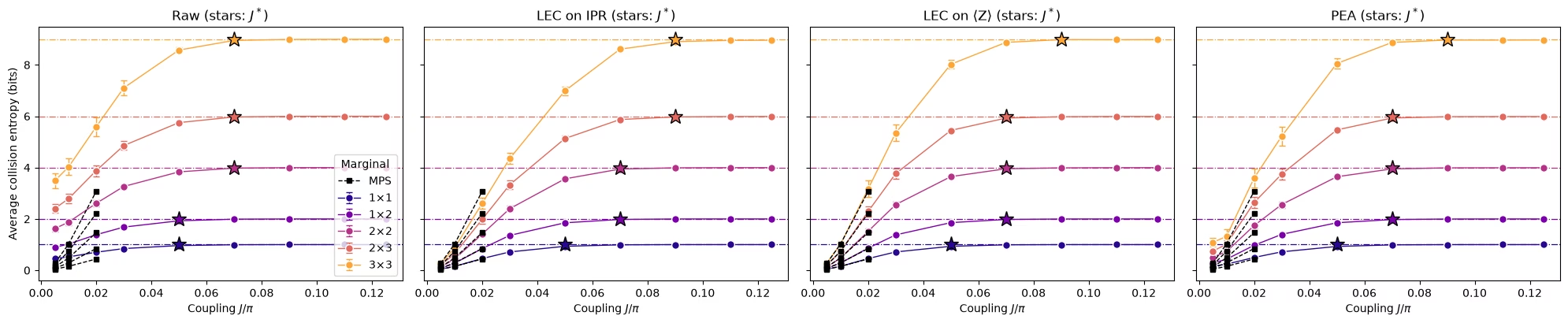
Lahat ng apat na estimate, at ang mga crossover
Kinakalkula ng susunod na function ang raw, LEC-on-IPR, LEC-on-, at PEA na mga estimate ng IPR ng isang posisyon ng marginal sa bawat coupling. Tinatantya rin nito ang shot noise ng bawat isa, sa pamamagitan ng pag-bootstrap sa mga randomization. Pinapatakbo ito ng cell para sa bawat placement na pumapasok sa mga average, na tumatagal nang mga isa't kalahating minuto.
def estimate_iprs(qubits, key):
    # Raw, LEC-on-IPR, LEC-on-<Z>, and PEA IPRs of one marginal position at every coupling,
    # with the shot noise of each from a bootstrap over the randomizations
    n = len(qubits)
    supports = parity_supports(qubits)
    # Parities with shape (noise factors, randomizations, supports), per coupling
    parities = [
        np.stack([parity_expectation_values(b, supports) for b in bits])
        for bits in raw_bits
    ]
    patch_bits = [
        bits[0][:, :, qubits] for bits in raw_bits
    ]  # noise factor 1
    values, errors = lec_estimates(
        patch_bits,
        [p[0] for p in parities],
        references[(calibration_hw, 64)][key],
        calibration_hw,
        n,
    )
    fidelities = np.array([readout_fidelity(s) for s in supports])

    def pea_statistic(p):
        return pea_ipr(p, fidelities, n)

    values["raw"] = [ipr_from_shots(b) for b in patch_bits]
    errors["raw"] = [bootstrap_error(ipr_from_shots, b) for b in patch_bits]
    values["PEA"] = [pea_statistic(p) for p in parities]
    errors["PEA"] = [
        bootstrap_error(pea_statistic, p, axis=1) for p in parities
    ]  # randomizations are axis 1
    return {m: np.array(v) for m, v in values.items()}, {
        m: np.array(e) for m, e in errors.items()
    }

methods = ["LEC on IPR", "LEC on ⟨Z⟩", "PEA"]
method_colors = {
    "LEC on IPR": "#2a78d6",
    "LEC on ⟨Z⟩": "#1baf7a",
    "PEA": "#eb6834",
}
iprs, ipr_errors = {}, {}
for label, patch_list in positions.items():
    for k in kept_placements[label]:
        iprs[label, k], ipr_errors[label, k] = estimate_iprs(
            patch_list[k], f"{label} {k}"
        )
print(f"{len(iprs)} clean marginal positions")
93 clean marginal positions
def crossover_coupling(couplings, entropies, haar, tolerance=0.1):
    # Smallest coupling whose entropy is within tolerance of the random-state value
    for coupling, entropy in zip(couplings, entropies):
        if entropy >= haar - tolerance:
            return coupling
    return None

def reference_ipr(index, chi, key):
    # IPR of the MPS distribution of a marginal
    return float((references[(index, chi)][key] ** 2).sum())

mps_settings = [
    (calibration_hw, 64),
    (1, 128),
    (2, 128),
]  # (coupling index, bond dimension)
panels = ["raw", *methods]

# Average IPR of every shape over its clean placements, then the entropy and the crossover
hw_entropies = {
    method: {} for method in panels
}  # per method and shape: average entropy and its error
crossovers = {method: {} for method in panels}
mps_entropies = {}  # per shape: MPS entropy, averaged over the same placements, at mps_settings
for label, patch_list in positions.items():
    haar = haar_entropy(len(patch_list[0]), num_qubits_hw)
    keys = [(shape, k) for (shape, k) in iprs if shape == label]
    mps_entropies[label] = [
        collision_entropy(
            np.mean([reference_ipr(j, chi, f"{label} {k}") for _, k in keys])
        )
        for j, chi in mps_settings
    ]
    for method in panels:
        ipr, ipr_error = average_ipr(
            [iprs[key][method] for key in keys],
            [ipr_errors[key][method] for key in keys],
        )
        entropy = collision_entropy(ipr)
        hw_entropies[method][label] = (entropy, ipr_error / (ipr * np.log(2)))
        crossovers[method][label] = crossover_coupling(
            couplings_hw, entropy, haar
        )
fig, axes = plt.subplots(
    1, len(panels), figsize=(5 * len(panels), 4.2), sharey=True
)
for (label, patch_list), color in zip(positions.items(), colors):
    haar = haar_entropy(len(patch_list[0]), num_qubits_hw)
    for ax, method in zip(axes, panels):
        entropy, error = hw_entropies[method][label]
        ax.errorbar(
            couplings_hw / np.pi,
            entropy,
            yerr=error,
            fmt="o-",
            color=color,
            mec="white",
            ms=7,
            lw=1,
            capsize=3,
            label=label,
        )
        ax.plot(
            couplings_hw[[j for j, _ in mps_settings]] / np.pi,
            mps_entropies[label],
            "s--",
            color="black",
            ms=4,
            lw=1,
            label="MPS" if label == "3×3" else None,
            zorder=4,
        )
        ax.axhline(haar, color=color, ls="dashdot", lw=0.9)
        if crossovers[method][label]:
            ax.plot(
                crossovers[method][label] / np.pi,
                haar,
                "*",
                ms=14,
                color=color,
                mec="black",
                zorder=3,
            )
for ax, method in zip(axes, panels):
    ax.set_title(f"{'Raw' if method == 'raw' else method} (stars: $J^*$)")
    ax.set_xlabel("Coupling $J/\\pi$")
axes[0].set_ylabel("Average collision entropy (bits)")
axes[0].legend(title="Marginal", loc="lower right")
fig.tight_layout()
plt.show()
Pagbubuod
Ang kinailangan para magpatakbo ng experiment na ganito kalaki:
-
Mga circuit na ang istruktura ay hindi nakadepende sa , na na-compile nang isang sublayer sa bawat pagkakataon, kaya isang noise model ang nagsisilbi sa buong sweep.
-
Mga estimator na gumagana mula sa mga bitstring: pair counting para sa IPR ng isang marginal, at ang Parseval form, na binabawasan ng variance ang bawat squared na parity, kapag mga na-mitigate na expectation value ang input.
-
Isang murang classical na angkla: ang ideal na state sa maliit na ang nagka-calibrate ng noise, at sinusubok ng mga held-out na coupling ang calibration. Ang hiwalay na pag-calibrate sa bawat , sa halip na sa IPR sa kabuuan, ang dahilan kung bakit nagkakasundo ang malalaking marginal.
-
Mga tool ng IBM para sa mabibigat na gawain: mga Samplomatic box at twirling,
NoiseLearnerV3, dynamical decoupling, at isangExecutorjob na may noise amplification para sa PEA. -
Mga pagsusuri sa kalidad ng data na data lang ang ginagamit.
Mga susunod na hakbang. Para lumalim pa sa mitigation, tingnan ang mga tutorial na probabilistic error amplification at PEC with shaded lightcones.